Author: Debanka

The File Controller allows you to send any type of file(s) from GTT to the device. It does not restrict file type or extension and allows file sizes up to 4GB.

The audio object is responsible for validating that the file being loaded is of the correct type. The file controller does not check the IDs used in audio objects.
Developers and system designers must verify the correct file type when using the file controller. For example, a configuration file should not be loaded into a file player, or a WAV file should not be used as an audio object configuration.
The audio object will return an error state if any invalid file type is detected, and this error must be handled appropriately.

The following are the options available in the file controller.

• Select Workspace
• Add Files
• Delete File
• Replace File
• Send to Device
• Verify Checksum
• Export Options
• Export and Import File Controller Data

The file controller feature is available from W release onwards.

Select Workspace

The Select Workspace option allows you to browse and select a workspace or root folder from the local directory. Once the folder is selected, you can add the respective audio files.

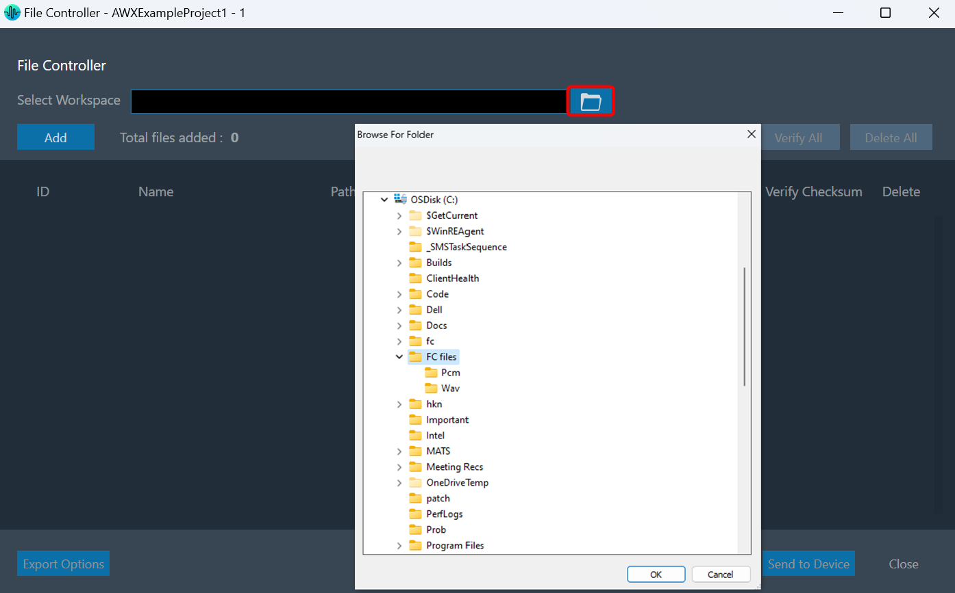
Also, you can copy and paste the path of your workspace folder in the “Workspace” field.

Add Files

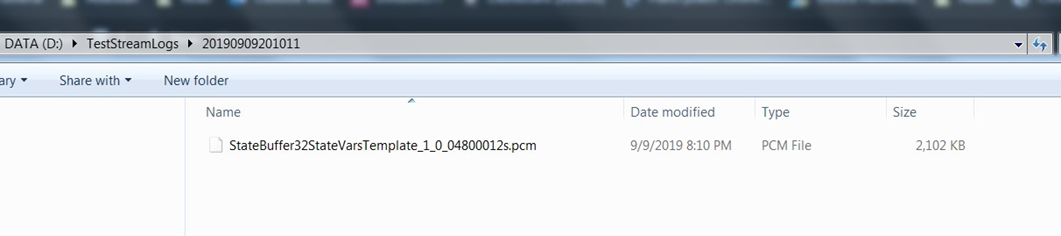
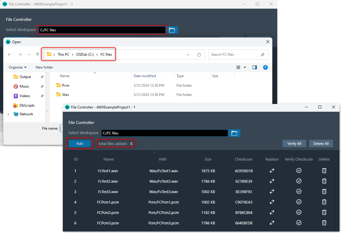
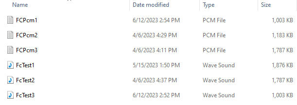
Once the workspace folder is selected, click on the “Add” to launch file browser. You can navigate to the respective folder and add audio files (.pcm/.wav) in file controller from the workspace folder.

The file browser will open the workspace folder by default.

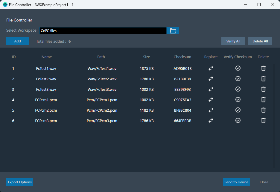
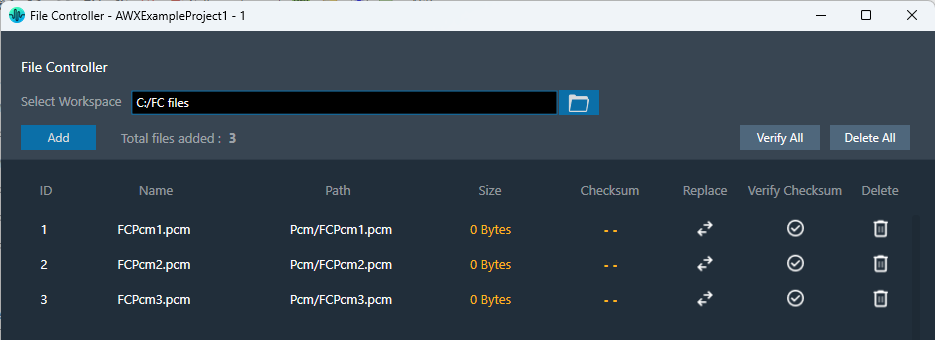
After adding the files, the following details of the files will be displayed in the file controller.

• File ID:  This ID is generated from GTT; its range is from 1 to 254.
• File Name: If the file name is exceeding length of 15 characters (including file extension), GTT will trim it to 15 characters.
• Path: Relative path of file, based on the workspace folder selected.
• Size: Size of the file in KB. If the file size is less than 1KB, the size will be displayed in bytes.
• Checksum: Checksum calculated using file content.

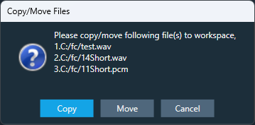
In case if you add any file from a non-workspace folder, the following prompt will appear.

• Copy: To create a duplicate copy of the file within your workspace folder.
• Move: To relocate the selected file to your workspace folder, removing it from its original location.
• Cancel: To stop the ongoing operation.

This facilitates the sharing of project files and files added to the file controller by ensuring that all files added to the file controller are present in the workspace folder.

The number of files added will be displayed in the File Controller.

A maximum of 254 files can be added in the file controller.

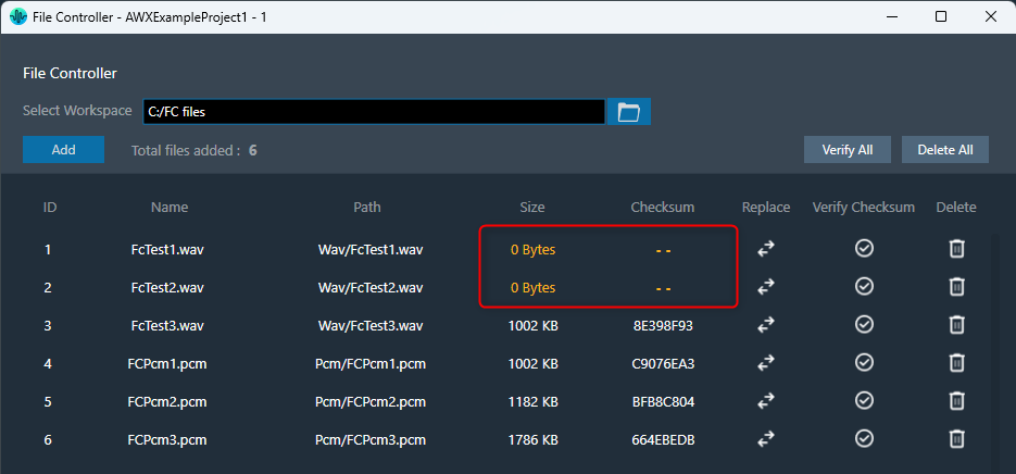
Once after adding files to the file controller, on relaunching the file controller, if any file is not found to load, the error is indicated by showing “0 Bytes” size and invalid checksum as below,

Delete Files

The file controller offers two ways to manage your files:

• Click “Delete All” to remove all files at once.
• Use the “Delete” button for each file to remove them individually.

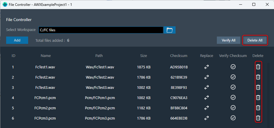
The delete operation will delete the file entry from the file controller, not the file from the file system.

Replace File

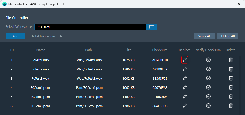
You can replace file in the file controller. Click on the “Replace” button, this will open the file browser, allowing you to select the new file you wish to use.
Also, allows you to reuse the file ID for different files easily.

Send to Device

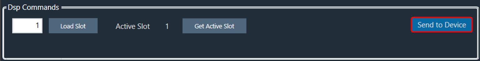
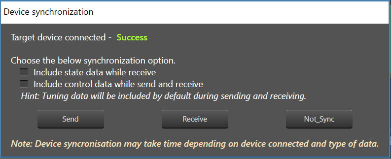
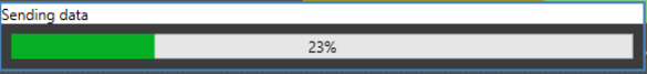
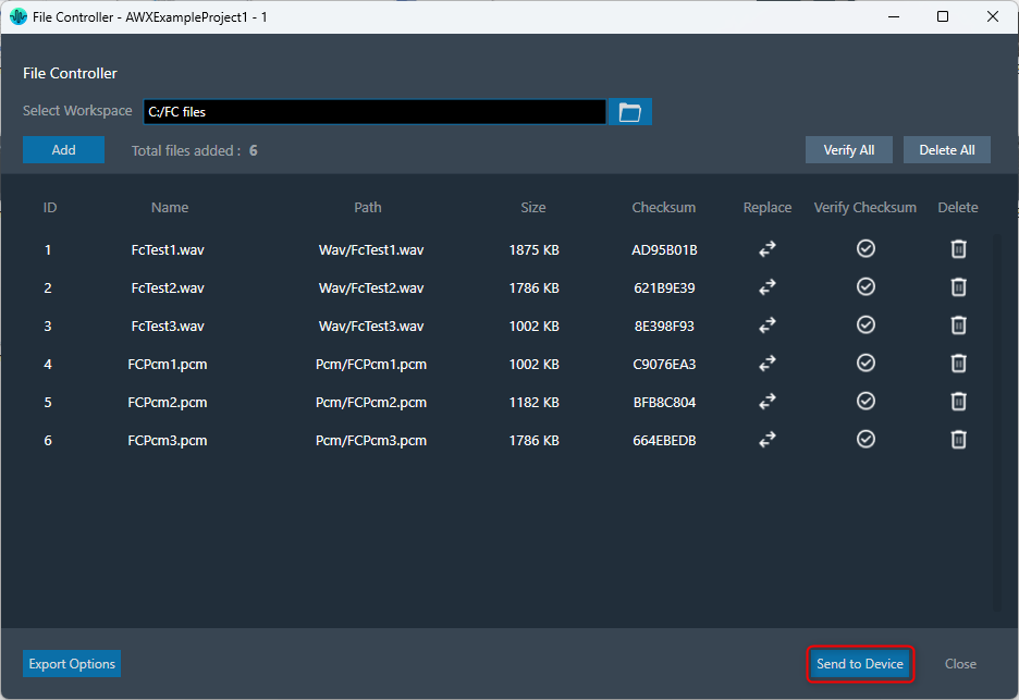
The “Send to Device” allows sending the loaded files in the file controller to the device.
While sending files to device, the file map will be sent to device first. It contains metadata (number of files and sizes) about the files being sent.
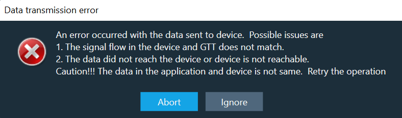
If it fails to send the file map, the files will not be transferred to the device.

Verify Checksum

The “Verify Checksum” feature helps ensure you’re working with the correct files. The Verify Checksum option uses the file content checksum to confirm that a file with the same file ID is present on the device.

Use the “Verify All” button to check all files at once, or the individual “Verify” button in each row for specific files.

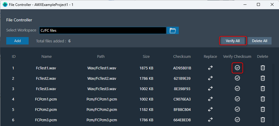
	Indicates the default state is “Not Verified”.
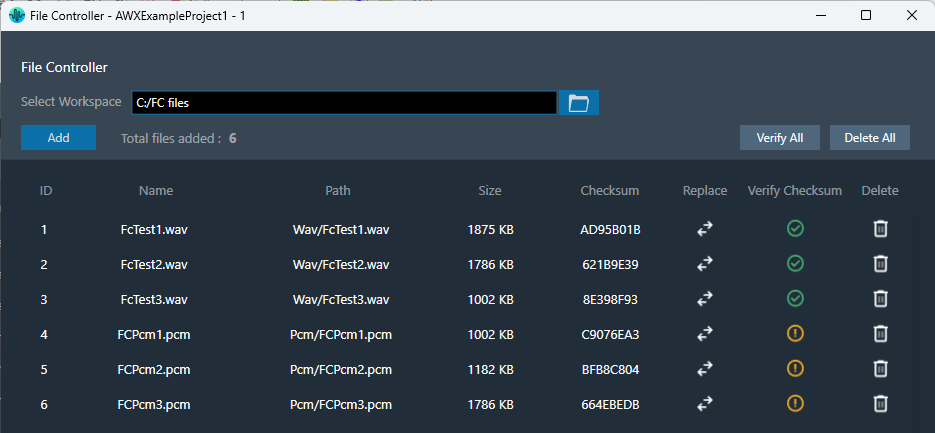
	Indicates when the file is found on a device with the same file ID. Also, when the file is sent to the device successfully.
	Indicates when the file is not found on the device with the same file ID.

Export Options

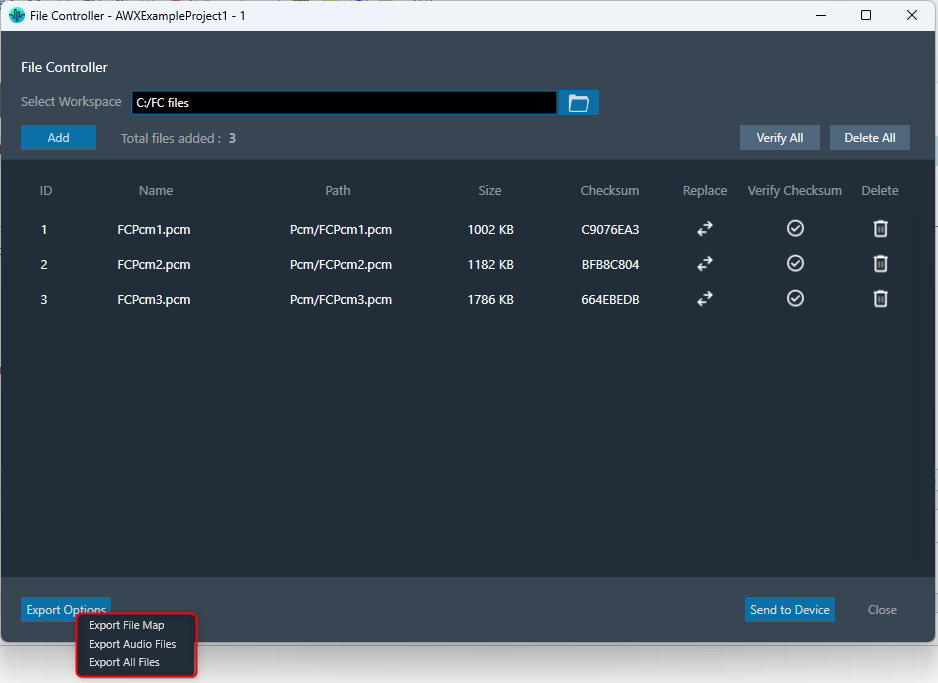
To export files from the file controller, the following options are available.

• Export File Map
• Export Audio Files
• Export All Files

These options will be displayed on clicking the “Export Options” button.

Upon selecting any of these options, a folder browser will open, allowing you to select the destination folder.

• Export File Map: This option is to export the file map and human-readable file map.
  
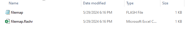
• Export Audio Files: This option is to export audio files added in the file controller.
  
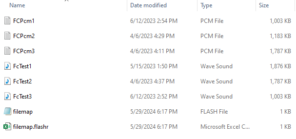
• Export All Files: This option is to export all files, including the file map and human-readable file map.
  

Export and Import File Controller Data

The selected workspace and metadata of loaded files in file controller can be exported through project file (.gttd). This metadata includes file ID, name and relative path of file. After importing the gttd file with file controller data, if the workspace folder is not found, files will be displayed with “0 bytes” Size and invalid checksum as shown below.

You can select workspace folder with same sub folder structure to automatically reload files loaded in file controller. The files should be present in same hierarchy and name.

Steps to send preset data online:

1. Connect to the device.
2. Click on Send To Device under the DSP Commands section. The Preset Configuration, Slot Map, and Presets are sent in sequence.

The default slot is the slot number loaded at boot. By default, it is set to “255:None”. You can specify the default loaded slot.

When loading the standard slot, the framework does not apply ramps

Once a preset has been flashed, it will not be flashed again, i.e. each preset configured in the slot map will only be sent once.

If any of these commands fail to be sent, the next command will not be sent, and an error message will be displayed.

When the preset data has been successfully sent, a completion message is displayed to indicate that the transmission was successful. If an error occurs, an error message is displayed.

Steps to connect a Device.

1. Navigate to the IVP RTA tab and select Advanced from the ribbon bar. This opens the RTA Settings dialogue box.
2. On the RTA Settings dialogue box, select the Plugins tab, and click on the folder icon to browse the xAF library path.
3. Set the port number under the Port box.
4. Enable the Bypass option (optional), if you prefer the input to be passed directly to the next plugin or output without undergoing any processing.
5. Click on Apply. The number of inputs, number of outputs, and plugin type will be automatically updated based on the provided signal flow. Similarly, you can set remaining plugins.
   Click on Reset (optional), to set back all the values in a specific row to their default values. Now you can configure the analyzer settings like the plugging host, Sound Card Settings, Generator Settings. For more information, refer to RTA Settings.
6. Switch to Device Designer tab and click on Connect Device to connect to device.
   
7. On successful connection with device the Device synchronization dialogue box will appear.

On the Device Synchronization dialogue box, you will get the below option.

• Send: Sends tuning data or control data from GTT to target device.
• Receive: Receives tuning data or control data from target device to GTT.
• Not_Sync: No exchange of tuning data between target device and GTT.

The Device Synchronization dialogue box also includes two check boxes.

• Include state data while receive.
  • If this option is checked and “Receive” operation is selected – The state data will be received from target device along with tuning data to GTT.
  • If this option is not checked and receive operation is selected – Only tuning data will be received from target device to GTT.
  • Checkbox value will be persist per device in GTT.
• Include control data while send and receive.
  • If this option is checked and “Receive” operation is selected – The control data will be received from target device along with tuning data to GTT.
  • If this option is not checked and “Receive” operation is selected – Only tuning data will be received from target device to GTT.
  • If this option is checked and “Send” operation is selected – Control data will be sent from GTT along with tuning data to target device.
  • If this option is not checked and “Send” operation is selected – Only tuning data will be sent from GTT to target device.
  • Checkbox value will be persist per device in GTT.

The selected data is stored and can be transferred using a .gttd file format for export and import purposes.

Switching off “Include state data while receive” during receive operation might impact synchronization of some audio object panels.

Sending or receiving data is indicated by a progress window along with a percentage of completion of sending or receiving data. The progress bar will close automatically once the send / receive process is completed.

The progress bar window title will be either “Sending data” or “Receiving data” depending on the functionality you have selected.

You can also perform “Send” and “Receive” operation from ribbon bar. To achieve this, the device should already be in a connected state. Following are the options provided as part of context menu.

• Send Tuning Data: Send tuning data will only send tuning data from GTT to target device.
• Receive Tuning Data: Receive tuning data will only receive tuning data from target device to GTT.
• Receive State Data: Receive state data will only receive state data from target device to GTT.
  

If EOC object is present in the signal flow, Progress window will not show the real progress.

In case there is issue with data transfer between device and GTT. a warning message appears asking you to abort or ignore the operation. You can check the device setup and retry the operation.

While sending the data from GTT to connected device, if there is a data transfer issue between the device and the GTT.  A warning will appear asking whether to abort the operation or ignore the error and continue.
You can troubleshoot the issue by verifying your device configuration and then retry the operation.

While sending the data from GTT to connected device, if there is a version mismatch between GTT and the connected device. A warning message will appears asking whether to continue or abort the operation.

Removing Device Instance

1. Select device and click on Delete. A warning message will be displayed.
2. Click OK to remove the device instance from the project.

Removing a device instance carries significant consequences, including the deletion of all associated data such as tuning and signal flows.

The streaming data can be recorded and stored in a file using the record button available. There are two supported file formats.

• Csv file format (.log)
• PCM file format (.pcm)

The default recording folder is C:UsersUsernameAppDataLocalHarmanGTTPCMStreamingLogs. To change the folder location for the recording, you need to click on “…” button.

Record Streaming Data in csv format

The csv format logs are supported by both polling and streaming state variables. Once you click on the record button, it opens file explorer to choose the location and file name for storing streaming data.

The default file format for storing streaming recordings is CSV.

The recording process is indicated by a continuously blinking button, indicating that streaming is currently being recorded. To stop the recording, simply use the same button.

During the recording process, adding or stopping streaming is not permitted.

The file stores the following information in the streaming data:

• Buffer Size and Update Rate.
• Streaming variables names with comma (,) separator.
• Streaming variable data with comma (,) separator and if any variables have an array of data it is separated by spaces.
  

Record Streaming Data in PCM format

The PCM format recording only supported by streaming state variable. Once you click on the record button, it opens file explorer to choose the location and file name for storing streaming data.
Prior to commencing PCM format recording, you must ensure the following conditions are met:

• The State Variable used for streaming is of a streamable type.
• PCM format is selected as the file format.
  

The recording process is indicated by a continuously blinking button, an indication that streaming is currently being recorded. To stop the recording, simply use the same button.

During the recording process, adding or stopping streaming is not permitted.

Each state variable’s streaming data is stored in a separate file containing raw data, which can be imported into tools such as Audacity for further analysis or processing.
A date-time stamped folder is automatically created for each recording under the root folder. Inside this folder, a separate file is generated for each state variable being streamed.

File Name Format: {state variable Name} {Channel Name} {Audio Object Name} {sample rate} {duration in seconds}. pcm

Example of sample recorded file.

Pause and Play Streaming

The streaming data can be paused by using the pause button. When the stream is paused, it indicates that GTT Tool stops receiving data from the device internally, and no bandwidth is utilized during this pause period.

To resume streaming, the same button can be used, and it will convert to a play button once data is paused.

It is not permitted to add new state variables or change the update rate while the streaming is paused. However, stopping an active state variable is allowed.

FFT Analysis capabilities are also available in the streaming window, wherein the FFT analysis of incoming audio signals is undertaken in real-time, depending upon the block size, additional calculations, etc).
The “Display Type” selection under the General tab provides the option to switch between Time and Frequency domain display.
When the Display Type is set to “Frequency Domain”, the Spectrum functionality of Streaming can be viewed.

In Spectrum view the X-axis ranges from “0 to Sampling Frequency / 2”, and Y-Axis ranges from “0 to -90 dbFS”.
Providing the correct sampling frequency is the responsibility of the audio engineer, and it should match the sampling frequency of the streaming state variable.
The Spectrum properties such as Block size, Sampling Frequency, Smoothing, and Averaging can be configured according to your requirements.

The variable “MaxWinSize” determines the maximum window size for smoothing in the Spectrum functionality. It has three options: Low (20), Medium (40), and High (1000). Choosing a larger number will result in a smoother curve.
For instance, if you set the limit to 500 Hz, all bins in the upper frequency range will be smoothed by averaging a window width of 500 Hz.

Example: Smoothing set to Off.

Example: Smoothing set to Low.

Example: Smoothing set to Medium.

Example: Smoothing set to High.

In GTT you can open multiple signal flow design simultaneously and tune the audio objects associated with different xAF Instances from either the same or different devices.

To open multiple signal flow design:

1. Right-click on any of the Xaf Instance and click Open signal Flow for Tuning.
   

This opens the signal flow designer in a separate floating window. Similarly, you can open multiple signal flow designer in a separate floating window and perform tuning operations.

The signal flow designer window can be identified by its title bar, which displays the name of the respective device associated with that window.
Device name -> Virtual core name -> xAF Instance name.

The Signal flow designer floating windows will be in read-only mode. In the read-only mode, you can search and select audio objects. Although you cannot make any modifications to the signal flow itself, you can navigate through the audio objects and tune them.

On the read-only signal flow designer floating window, double-click on the audio object to view their properties and launch corresponding panels. This functionality enables you to perform tuning operations on multiple signal flows simultaneously.

You can either copy partially or complete signal flow from read-only mode and then paste it into editable signal flows.

Tuning Compound Audio Object in Multiple Signal Flow Design

If the signal flow contains instances of compound audio object (CAO), you can open the signal flow of the compound audio object by selecting it from the context menu. This allows you to perform tuning on the inner audio objects of the CAO as well as apply tuning data specific to the preset type of the compound audio object.

When device is connected, then processing state can be set from all opened signal flows.

When probe-points are enabled for the core, you also have the option to add, remove, enable, or disable probe points.

To modify the properties of the device core or core object, it is necessary to close any open signal flows associated with them. A confirmation message will appear and selecting “Ok” will close all signal flow windows related to the chosen device. If “Cancel” is clicked, the property change will be aborted.

GTT provides an option to use file-based devices. A default custom file with file extension .deviceInfo  available under Devices folder (C:Program FilesHarmanHarmanAudioworXtoolsGTTDevices).

Also, you need a .ddf  file, which you can keep under the Custom Device folder.

You can create a .ddf  file in GTT. Once you have created a project, click on the Export option, and select DDF Data. Now browse to C:Program FilesHarmanHarmanAudioworXtoolsGTTDevicesCustomDevice location and save the file.

Once the above files are placed in the folder. The custom device will be shown in the Devices view tab in GTT. You can drag-drop this device into the venue explorer. This is similar to any other device created inside GTT.

This file-based device has some limitations. In the normal device (created inside GTT), double-click will open the signal flow designer. But this is not the case with custom devices. This device is not stored in a database. So, the signal flow designer will not be opened.

It is possible to create a custom panel and use the device. However, because it is a file-based device, it is not stored in the GTT database. To reuse the project, export it as a file and then import it whenever needed.

The custom devices created will not be part of the existing project as the devices displayed in the location are retrieved from the GTT database, and custom devices are not stored in the GTT database.

Regardless of the sorting order, the Add Device Dialog always displays the Custom Device as the top option if it is available.

The Custom Device is loaded when the application is launched. Therefore, if any changes are made to the associated .DDF file after launching GTT, it is necessary to relaunch GTT and add the custom device again to ensure the modifications are reflected.

The source for the Custom Device is the .DDF file, which launches the State Variable window. This window displays the audio object definitions that are contained within the associated .DDF file and these definitions can be utilized during panel designing.

When working with multiple xAF audio library versions (DLL version) in GTT, any new device added to the project will be automatically linked with the default audio library version (DLL version).

If the linking of existing devices with their respective DLLs was done in the “O” version of GTT or if the DLLs were loaded before the project was imported to GTT, those devices will still function with their respective DLLs without any issues.

On the property view of the device instance, you can see the audio library version of the respective device.

Changing Device Audio Library

To change the audio library version of the device:

1. On the device view, click on the Audio Library Version. This opens the property view of the device.
   
2. Select the desired DLL version from the drop-down, and click Save.
   

The device will start working with the updated DLL version.

If a device has a signal flow with audio objects created in a previous version, compatible audio objects are automatically upgraded.

Once you update the DLL version, if any non-compatible audio objects are there, it will be highlighted in blue and the warning displayed in the compiler report.

You can fix the non-compatible audio objects in the signal flow. Right-click on the highlighted audio object and select upgraded audio object from the context menu.

Change of association DLL for one device will not impact other device instance.

xAF Audio Library Use Cases

While importing a project file in GTT, make sure the xAF audio library version is already available in GTT.

• Use Case 1: When you import a project, if the xAF DLL associated with the project is already loaded in the GTT audio library. Regardless of whether the associated DLL is the default library or not, the project will import without error or warning. Later, you can switch to the latest DLL.
• Use Case 2: While importing a project, if the xAF DLL associated with the project is not loaded in the GTT audio library, then the project will be linked to the default xAF DLL in GTT.

When you open the project after importing it, a message will appear. This displays the default audio library of project and details of previous audio library that is associated with the imported project.

Once you open the Signal Flow Designer of the imported project, the below message will appear every time you open the Signal Flow Designer of the project.

You can get rid of the message by using the methods listed below.

• Once you open the Signal Flow Designer of the project, go to the non-compatible audio objects, which are highlighted in blue. Right-click on the highlighted audio object, select upgraded audio object from the context menu, and save the changes. This will upgrade the non-compatible audio objects in the project.
• The message will not appear if you import the previous DLL (which is associated with the imported project) into the GTT audio library manager.

Use Case 3: While importing a project, if the xAF DLL associated with the project is not loaded in GTT audio library and the default xAF DLL is not compatible. An error message will be displayed, and project import will be cancelled.

Use Case 4: After importing a project and switching to a different audio library, you may encounter missing audio objects in the Signal Flow Designer. These missing objects will be highlighted in red, and an error message with a list of the missing audio objects will be displayed. The same error message will also be included in the compiler report.

In order to resolve the error, it is necessary to delete the missing audio object from the Signal Flow Designer. Once the missing audio object is removed, the error will be cleared.