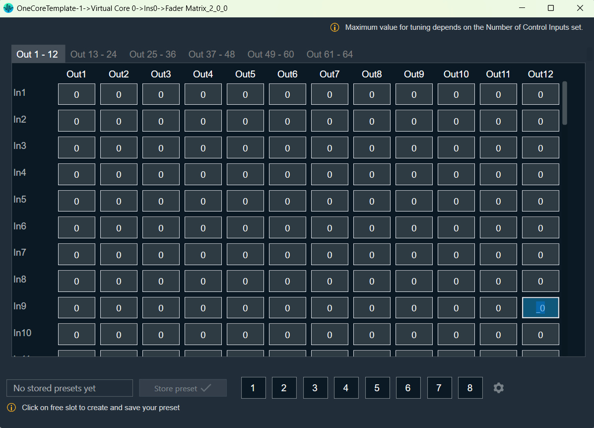
The Fader Matrix panel is a table panel with rows and columns to tune the state variables for the Fader Matrix audio object.
The Fader Matrix Panel features a configurable number of input and output channels, which correspond to the rows and columns, respectively. The dimensions of the Fader Matrix Panel—namely, the number of rows and columns—are determined by the values set for the ‘Audio In’ and ‘Audio Out’ properties of the Fader Matrix Audio object.
The maximum number of input channels, output channels, and control inputs that can be configured is 64.

The Fader Matrix panel window has tabs for grouping output channels sequentially, where each tab displays 12 channels.

Tuning Fader Matrix AO

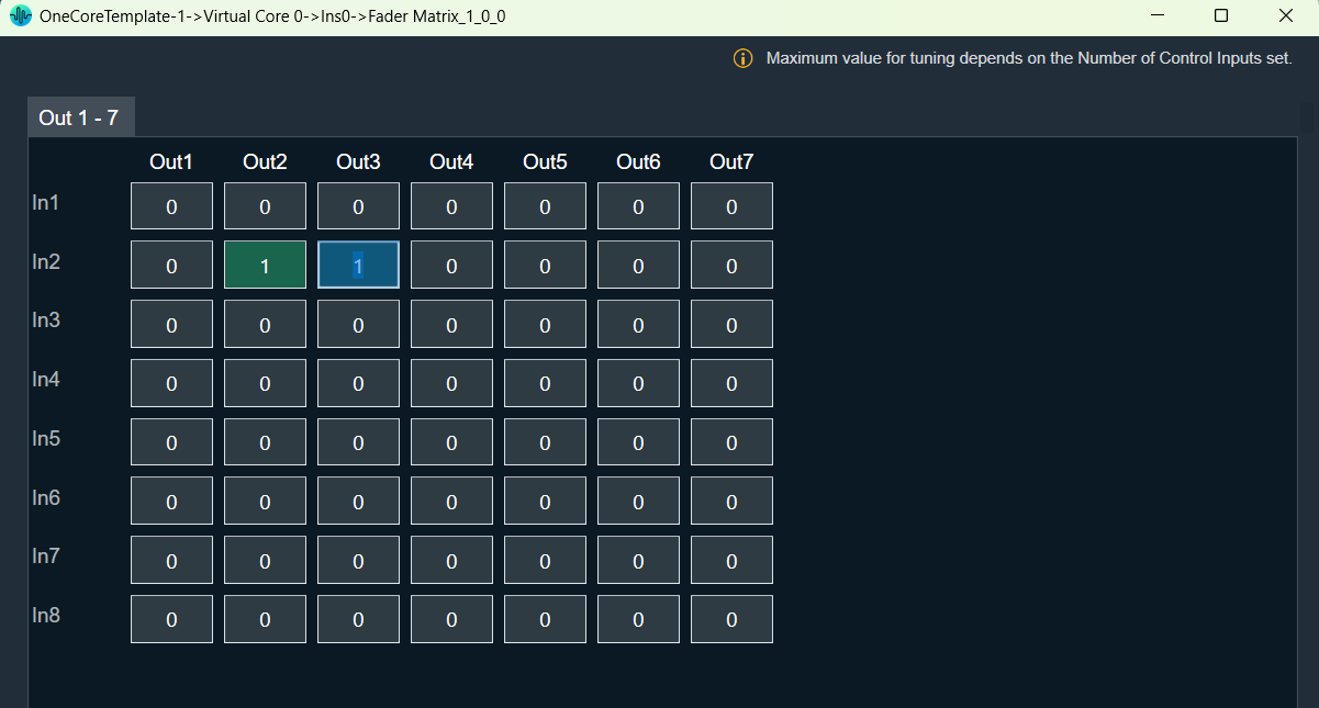
The minimum value that can be tuned for the Fader matrix audio object is 0, which is the default value.
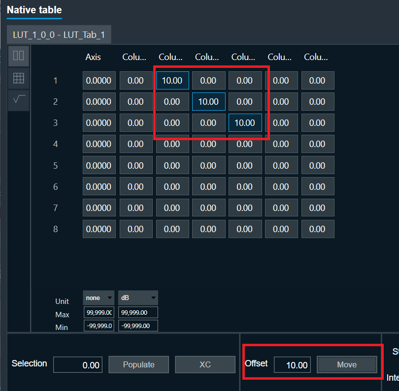
The maximum tuning value is determined by the ‘Number of Control Inputs’ property of the fader matrix audio object. The tuned cells are highlighted in green to distinguish them from untuned cells. Additionally, you can perform Cut, Copy, Paste, Delete, Undo, and Select All operations on the text values of the fader matrix panel cells using a context menu.

Cell Selection Methods

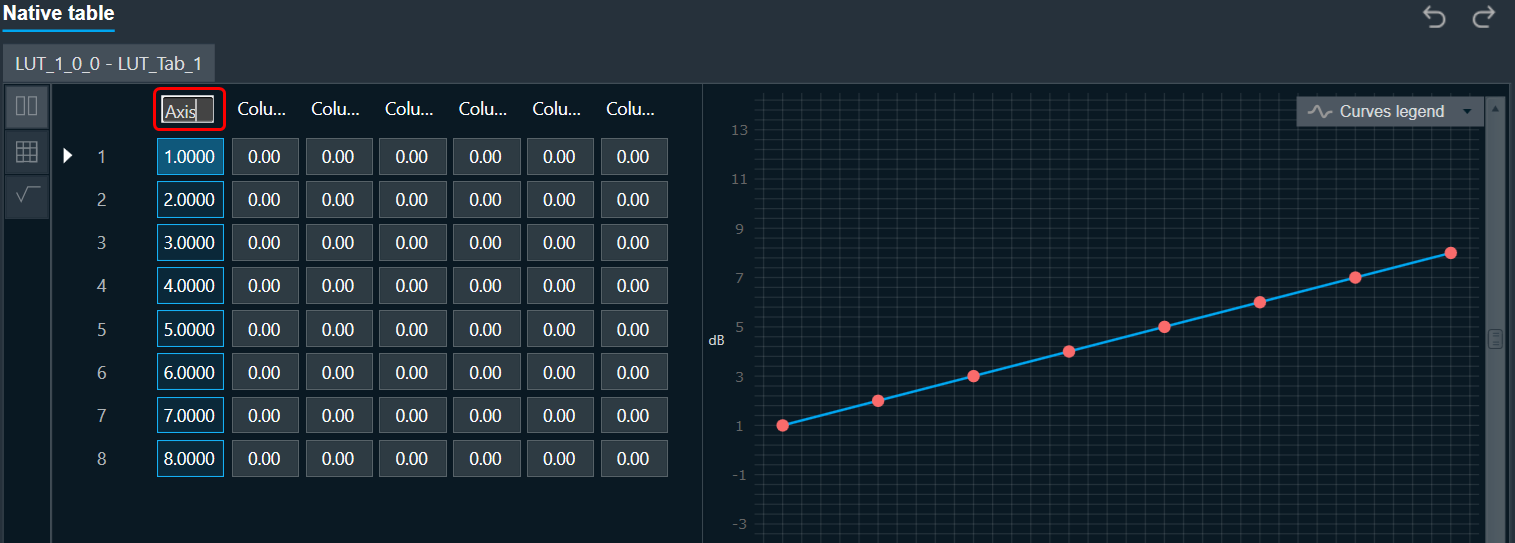
• Single cell selection method: You can select a single cell using the mouse by left-clicking or by pressing the tab key on your keyboard. Once selected, the cell will be highlighted, as shown in the example below. The text within the selected cell can be edited.
  
• Multiple cell selection methods: There are two ways to select multiple cells.
  • Method 1: By clicking and dragging with the mouse. This method is useful when you are selecting a small range of cells.
  • Method 2: By using keys on the keyboard. This method is useful when rendered outside of the view area when the grid scrolls either vertically or horizontally.

Method 1

Method 2

To select multiple cells using the mouse, follow the steps below. Place the cursor on a cell. Select the cell by using the left mouse button and keeping the mouse button pressed. Drag the cursor in the respective cell. Automatically, the cells will be selected in matrix form. Leave the mouse button. The selected cell will be highlighted as you can see in the example below.

To select multiple cells that are rendered outside of the view area when the grid scrolls either vertically or horizontally, you can use the method below for selecting multiple cells. If you want to select a cell that is rendered outside of the view area when the grid scrolls either vertically or horizontally, you can use the method below for selecting multiple cells. Click on the first cell of the range. Use the scroll bar to navigate to the last cell of the range. Hold the Shift key and click on the last cell of the range. This will automatically select every cell in the matrix form. The selected cell will be highlighted as you can see in the example below.

Selecting arbitrary cells is not allowed. Selection is always in the form of a matrix.

The selected region is reset and not tracked when changing tabs.

Copy and Paste Functionality

You can copy and paste the factor matrix table data into Excel or vice versa. There are several methods for copying and pasting data.

• Method 1: To copy panel cell data to Excel.
• Method 2: To copy data from Excel to the factor matrix table.

Method 1

Method 2

To copy panel cell data to Excel. Place the cursor on the cell, select the cell by using the left mouse button, and keep the mouse button pressed. Drag the cursor in the respective cell. Automatically, the cells will be selected in matrix form. Press Ctrl + C on your keyboard. The content gets copied to the clipboard. Switch to Excel spreadsheet. Press Ctrl + V on your keyboard in the desired location within your Excel spreadsheet.

To copy data from Excel to the factor matrix table. In your Excel spreadsheet, use the cursor on the cell to select the respective cell from Excel. Press Ctrl + C on your keyboard. This copies the data from the selected cells. Switch to fader matrix table. Choose the cell and press Ctrl + V.

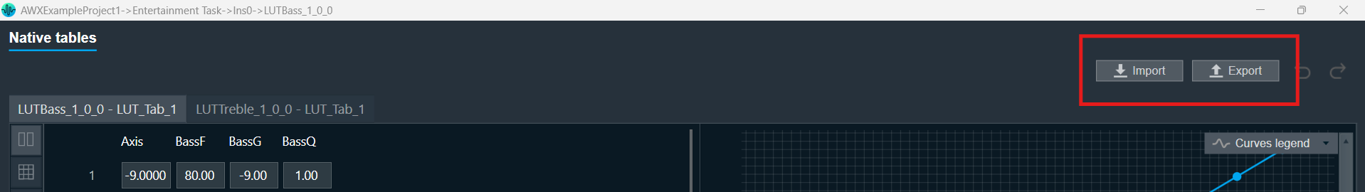
Preset Store Functionality

You can save and retrieve a specific configuration using the Store Preset option on the panel.
To do this, configure the tuning parameters, choose an available preset slot, enter a name for the slot, and click on Store Preset. This will save the current tuning data for the selected slot.

If you do not enter a name of the slot, then it will take the default name “New Preset”.

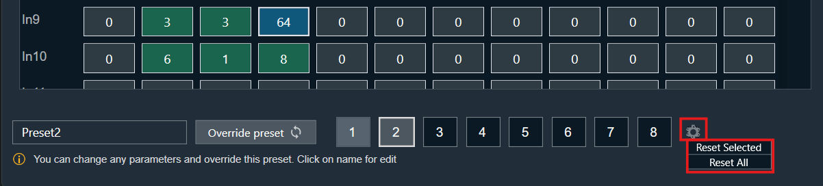
You can switch between preset slots and apply their values by simply clicking on them. Additionally, after clicking to override the preset, you can modify the tuning values in that tab or change the preset name.

To reset the selected preset or all the preset values.

• Click ResetSelected to clear the preset that is currently selected.
• Click Reset All to clear every preset in the corresponding native panel.
  
  

The Limiter object can be used to create a hard-stop peak limit on an input signal.  Because it operates on a feedback basis only, there is the possibility for the input signal to overshoot the limit set by the user for a short duration while the algorithm pulls down the signal gain.

The basic trade-off of any feedback limiter is strict regulation to the threshold versus distortion. The more aggressively the limiter is working to pull down (attack) the signal level to the threshold, the more distortion will be produced. Distortion, fluttering and/or pumping can also be produced when the signal level is released from regulation, if the resulting gain lift happens too fast.

Limiter Operation Description

• Attack Phase – When the Limiter detects that the Threshold value has been exceeded, it reduces the gain at a rate set by a combination of the Attack parameter and how much the input signal exceeds the Threshold value. The gain is reduced until the signal level is at or below the Threshold value. The faster the gain is reduced, the more distortion will be created. There is a minimum attack time time period during which the algorithm is determining signal level.
• Hold Phase – After the signal drops below the Threshold value, the Limiter will hold the gain steady for a time determined by the Hold parameter. It stops the gain reduction phase and begins to hold. Then at the point when the signal has fallen below the Hold threshold value, the Release phase begins.
• Release Phase – The gain is raised back to the starting gain, set by the Gain parameter, at a rate determined by the Release parameter. The faster the gain is raised, the more distortion will be created.

Limiter Tuning Parameters In-Depth Description

• Gain – this is a gain stage before the limiting portion of the algorithm, which sets the starting gain. This gain is applicable before limiting starts, after limiting is fully released and while no limiting is occurring. Gain changes during limiting will be added to this value.
• Threshold – this is the peak level under which the Limiter will attempt to keep the signal. Overshoot can happen during the Attack phase, both while the algorithm is computing signal level and while reducing gain to meet the Threshold value.
• Hold Threshold – this is the signal level, relative to the Threshold value, under which the Release phase will begin. This small offset keeps the algorithm from changing phases too quickly and provides an extra guard against exceeding the Threshold value, helping to reduce fluttering and distortion.
• Attack Time – this is how fast, and thus how aggressively, the Limiter will pull down the signal to meet the threshold. If strict adherence to the Threshold parameter is desired, then Attack should be set very low. This will produce more distortion than a more relaxed Attack value, but if the input signal is not anticipated to exceed the Threshold by very much, then the distortion will be relatively low. Worst case is when the Attack is set low and the input signal level is high compared to the Threshold value. There is a minimum attack time the user can set, which corresponds to the time period during which the algorithm is determining signal level.
• Hold Time – this sets the time during which the Limiter will hold the gain value steady. Having a non-zero value here can smooth the Limiter operation so that fluttering and pumping are less audible.
• Release Time – this sets the time during which the Limiter will begin raising the gain back to the original value. Extremely short release times cause very fast gain changes which can lead to fluttering, pumping and distortion.

About Biquad Topology

• Direct Form I (DFI)
• Direct Form II (DFII)
• Transposed Direct Form II (TDFII)

Direct Form I (DFI)

Structure: The DFI structure implements the zeros of the transfer function first, followed by the poles. It uses two separate delay lines for the input and output signals.

Direct Form II (DFII)

Structure: The DFII structure rearranges the DFI structure by using a single delay line for both the input and output signals. It implements the poles first, followed by the zeros.

Advantages

Disadvantages

Memory Efficient (Canonical Form): It is a canonical form, meaning it uses the minimum number of delay elements required for a second-order filter. Potentially Faster Code Execution: Some implementations might lead to slightly faster code compared to DFI.

Higher Risk of Overflow: The poles are implemented first. If the filter has a high Q-factor or gain near the resonant frequency, the internal signal levels in the delay line can become very large, leading to overflow, especially in fixed-point implementations. More Sensitive to Quantization Noise: Quantization errors introduced within the feedback loop are directly fed back and shaped by the poles, potentially leading to more noticeable noise. Poor Parameter Modulation Behaviour: DFII is known to produce artifacts like clicks and pops when filter parameters are changed rapidly due to the high gain that can occur in the state variables.

Transposed Direct Form II (TDFII)

Structure: The transposed form of DFII is obtained by reversing the signal flow graph. Branch points become summers, and summers become branch points. The transfer function remains the same. It also uses a single delay line.

Advantages

Disadvantages

Memory Efficient (Canonical Form): Like DFII, it is also a canonical form with minimal delay elements. Lower Quantization Noise: Generally considered to have better numerical properties and lower quantization noise compared to the direct forms, especially in floating-point implementations where each multiplication and potentially each addition is rounded. Better Robustness: It often exhibits robustness similar to DFI in terms of handling internal signal levels compared to the direct DFII. The zeros are effectively implemented before the feedback path influences the output. Preferred for Floating-Point DSP: Due to its better noise characteristics, it is often preferred in floating-point digital signal processing.

Longer Critical Path: Similar to DFI, the transposed structure can have a longer critical path through the feedback loop, potentially limiting the maximum clock rate in hardware. Can be Less Intuitive: The transposed structure might be less directly related to the standard difference equation, making the implementation and analysis slightly less intuitive. Potential for Limit Cycles: In fixed-point implementations, transposed forms can sometimes be more prone to limit cycles (self-sustained oscillations at low levels) under certain conditions.

Summary

Feature	Direct Form I (DFI)	Direct Form II (DFII)	Direct Form II Transposed
Memory Usage	High	Low (Canonical)	Low (Canonical)
Overflow Risk	Lower	Higher	Moderate
Quantization Noise	Potentially Higher	Higher	Lower
Computational Cost	Moderate	Moderate	Moderate
Critical Path	Longer	Shorter	Longer
Parameter Modulation	Better	Poor	Good
Fixed-Point DSP	Good (with double acc.)	Can be problematic	Generally Good
Floating-Point DSP	Acceptable	Acceptable	Preferred

The Control demux audio object routes the input control signal to one of the control outputs based on the index value.

Control Demux Properties

The table below describes the audio object properties and functionalities.

Properties	Description
Number of ControlOuts	Enter the number of control outputs. Range: 2 to 255 Default: 2
Display Name	Display the name of the Control demux audio object in the signal flow design. It can be changed based on the intended usage of the object.

Mode

There are currently no modes available for the Control demux audio object.

Additional parameters

There are no additional parameters available for the Control demux audio object.

Tuning Parameters

The output index, which selects the control output through which the control input will be routed, could be changed as a tuning parameter.

Parameter	Description	Data Type	Range	Default	Unit
Output Index	Selects the output through which the input will be routed.	Unsigned Int	0 – (Number of control outputs -1)	0	none

Control Interface

There are two control inputs for the Control demux.

The first receives the control input. The second selects the control output through which the input will be routed.

Name	Description	Data Type	Range	Unit
Control Input	Receives the control input.	Float	Min: single precision float minimum -3.402823 x 10^38 Max: single precision float maximum 3.402823 x 10^38	None
Output Index	Selects the output through which the input will be routed.	Float	Min: 0 Max: Number of control outputs – 1	None

Native Panel

Control demux audio object does not support a native panel.

For all Audio Objects, inside their respective tuneXTP() methods, the received tuning data is NOT checked for valid range limits.
– If the Audio Object (AO) is tuned from GTT, the GTT ensures that the tuning parameters remain within the range prescribed by the toolbox methods.
– If the Audio Object (AO) is tuned using methods other than GTT, like SVE or xTP tuning, it is the responsibility of those entities to ensure that the tuning parameter values remain within the valid range as mentioned in the Audio Object Description User Guide.

All audio objects describe their features, attributes and capabilities to the tuning tool through meta data that are used in signal flow design.
The list of supported core types by each audio object is one among them. If the list is empty, it indicates that there are no restrictions and the audio object is supported on all core types.

The Control Generator audio object allows to generate a constant control value at a specified time.

Control Generator Properties

Below table describes the audio object properties and functionalities.

Properties	Description
# of  Control outputs	Enter the number of control outputs. In Single control mode, the number of control outputs is configurable between 1 to 255. In Multi control mode, the number of control outputs is the same as the number of control inputs. Range: 1 to 255 (Min – 1 and Max – 255) By default, the number of output channels is set to 1.
Display Name	Display the name of the Control Generator audio object in signal flow design. It can be changed based on the intended usage of the object.
Object Mode	This audio object can be configured in two operation modes. Single control Multi control

Mode

The object operates in one of the following two modes:

Mode	Description
Single control	In this mode, the object has a single control input and configurable control outputs ranging from 1 to 255. It has a single set of tuning parameters that decide the functioning of all control outputs. Based on the Control value and Trigger time configured, which is applied to all the control outputs,  the constant control value is sent out every “n” seconds i.e. trigger time configured. If its value is 0 the control value is sent out just once. This is the default mode.
Multi control	This audio object can be configured with control channels ranging from 1 to 255. The number of control inputs will be equal to the control outputs. The object has a separate set of tuning parameters that decide the functioning of each control output. Control value and Trigger time can be configured separately for each control output. The default number of control channels shall be 1.

The control input in both modes is triggered only and the value at the control output is set by the Control value tuning parameter.

Additional parameters

There are no additional parameters available for the Control Generator audio object.

Tuning Parameters

The following are the paraments that can be tuned from GTT.

Parameter	Description	Data Type	Range	Default	Unit
Control Value	The value which is sent out to the control output. Setting this value will send the constant control value out.	xFloat32	Min: single precision float minimum -3.402823 x 10^38 Max: single precision float maximum 3.402823  x 10^38	0.0f	NA
Trigger time	It is the rate at which the control value is sent on the control output. Setting this tuning parameter shall send the constant control value out. If its value is 0 the control value is sent out just once. If its value is greater than 0, let’s say a value of N, the control value shall be sent out every N seconds.	xFloat32	0 – 600	0.0f	seconds

Control Interface

The Single-control mode has a single control input and configurable control outputs. The control outputs are configured using the “# of Control outputs” property.  The control output value ranges from 1 to 255.

By default, control input and control output is 1.

The Multi-control mode has configurable control outputs. The control outputs are configured using the “# of Control outputs” property.  The control output value ranges from 1 to 255.
The number of control inputs is equal to the control outputs.

Native Panel

The Control Generator audio object does not support a native panel.

This guide explores a comprehensive library of audio algorithms from Harman. It includes over 90 algorithms that can be used to create new, flexible audio processing units (Compound Audio Objects). These CAOs can be fine-tuned, protected with passwords, and shared as easily as any individual audio object.

The audio objects are categorized into the following groups in the GTT.

The Rate Control audio object controls the rate at which control signals can pass through the object. This is implemented by blocking the controls for a duration that is specified as a tuning parameter.

Rate control Properties

Below table describes the audio object properties and functionalities.

Properties	Description
Number of controls	Enter the number of control inputs. The number of control outputs is always 2. The index of the pin (which receives the first control signal) is sent out on the left output pin first and then the control signal itself is sent on the right output pin. Range: 1 to 255 Data type: xFloat32 Default: 1
Display Name	Display name of the Rate control audio object in signal flow design. It can be changed based on the intended usage of the object.

Mode

There are currently no modes available for the Rate control audio object.

Additional parameters

There are no additional parameters available for the Rate control audio object.

Tuning Parameters

There are blocking times associated with each control input pin which could be changed as a tuning parameter.

Parameter	Description	Data Type	Range	Default	Unit
BlockingTime	Time for which any new control signal is blocked	xFloat32	0 – 60	0	seconds

Control Interface

The object supports configurable number of control inputs ranging from 1 to 255. The default number of control input is 1. The objects supports two control outputs.

Native Panel

Rate control audio object does not support a native panel.

The LUT object supports native panel.  Double-click on the LUT object to open the native panel and set the values accordingly.

• Redo/Undo: The redo and undo functions enable you to rollback or repeat the modifications made to panel cell values, units, minimums, and maximums.
  
• Customizable Axis Label: The customizable axis label allows you to change the axis label name. Double-clicking on the axis label will show a textbox where you can change the axis label name.
  
• Offset: An offset value is a number added or subtracted from selected cells.
  
• Export: Using the export option, you can export the currently opened LUT tab data into .csv format.

Only tuning data will be exported. Unit Type, Min, and Max values will not be part of the export.

• Import: You can import LUT data into the application using a .csv file. This feature allows you to reuse exported files or import externally computed data.
  The file must follow the validation rules below before import.
  • The file must be in .csv format.
  • The file must contain the same number of rows and columns as the currently opened LUT tab.
  • The first column must represent the Axis, and its values should be in ascending order.
  • All cell values in the file must be within the defined unit’s minimum and maximum limits. Once the import is successful, the Undo button will be enabled, allowing you to revert the import operation if necessary.
    

Fast Conv filter native panel allows you to configure the Mode of each enabled filter and to load coefficients as well. In order to see the graphs, you need to import coefficients. Use ‘Import’ or ‘Import All’ option to import coefficients.
To open the native panel, double-click on the Fast Conv filter audio object in the signal flow designer.

Amplitude/Phase: When the coefficients are given and “Amplitude/Phase” option is selected, the graph display the value.

Coefficients:  When the coefficients are given and the “Coefficients” option is selected, the graph displays the values as per below figure. You can change the graph style using the “Chart Style” option.

Line chart style: when “Chart Style” selected as Line, the Coefficients graph.
Dot chart style: when “Chart Style” selected as Dot, the Coefficients graph.

Group Delay: When the coefficients are given and “Group Delay” option is selected, the graph display the values.

Curves Legend: This option allows you to show the details of which graph tab (Amplitude/Phase, Coefficients, Group Delay) is selected.

On the selection of Amplitude/Phase graph tab Curves Legend will show below information.
On the selection of Coefficients graph tab and Chart Styles ‘Dots’, Curves Legend will show below information.
On the selection of Coefficients graph tab and Chart Styles ‘Line’, Curves Legend will show information.
On the selection of Group Delay graph tab, Curves Legend will show information.

Additional Functionalities

• Flat: This is used to make the graph flat by making coefficients to 0.
• Import: This function is used to import the coefficients for a single active filter. Click the “Import” button, then enter the file path and click Ok.
  All coefficients for the selected filter will be imported, as shown in the graph. If the number of coefficients does not match the number of taps as shown in the screenshot below, a warning pop up will appear.
  Click ‘Yes’ to import available coefficients or click ‘No’ to cancel the import.
• Export: This option is used to export coefficients for selected active filter into csv file.
• Export All: This option is used to export all active filters in one go. Click the “Export All” button, then enter the path and file name, then click Ok. A xml file will be created which will have coefficients for each active filter.
• Import All: This option is used to import all coefficients in one go. Click the “Import All” button, then enter the XML file path and click Ok. All the given coefficients will be imported and can be seen in the graph.
• Read:  This is used to read from the target to display in the panel.
• Send: This is used to send the values changed in panel to target.