Traces can be analyzed in RTA even if the sound card is not connected. If no sound card is assigned for the input and output channels, RTA will switch to offline mode, allowing you to analyze the captured traces.

In offline mode, there are limited options for analyzing captured traces. The following options can be used for analyzing captured traces while in offline mode.

On the Ribbon bar

• Analyzer Settings
• Advanced Settings
• Options to Save
• Load RTA Settings

Under the Advanced Settings window

• Graph Settings
  

The soundcard status is displayed in RTA using a green and red indicator.

• When the assigned sound card is available and connected.
  
• When the assigned sound card is unavailable, or sound cards are not assigned to the input and output channels.
  

The last applied RTA settings will be retained and available on connecting the assigned sound card.

The Probe Point functionality facilitates the streaming of data from any stage of the signal flow to GTT, enabling the analysis, recording, or reuse of the data within IVP. The primary purpose of this feature is to provide the capability to receive data from an audio object and perform real-time analysis of audio input using the Real-time Analyzer view.

Related Topics

• Configure Probe Point
• Manage Probe Points
• Device Reboot

Configure Probe Point

To enable probe points per core:

1. Open the Device View and select the Virtual core layer of the device.
2. Go to the Virtual core properties, select the Streaming checkbox, and set a number of probe points per core.

Only the configured number of probe points can be enabled in signal flow per core.

The configured probe points will be sent to the device using the “Send Device Config” feature. This configuration can be fetched from the device using the “Load Device Config” feature.

In order to utilize streaming for state variables, it is necessary to enable this feature. However, considering its resource-intensive nature, this high configuration feature can be skipped to ensure optimal utilization of MIPS and memory. The count of probe points specifically pertains to audio streams and a maximum of 16 probe points are supported for a core.

If Streaming is disabled for the core, the number of probe points input field will be disabled, and streamable state variables will be excluded for that core in the streaming window.

Add Probe Point

The Probe Point context menu for selected connections has the below options:

• Add: The feature allows you to add a probe point on a selected connection source point. Additionally, the default state of the probe point is set to the enabled state.

To add a probe point on the virtual connection:

• Right-click on the virtual connection > Probe Point > select Add.
  
  After adding probe points, the source point pin connection will be visually highlighted with a bright purple-colored icon.
  

Remove Probe Point

• Remove: You can remove a probe point from the selected connection.

To remove the probe point from the virtual connection:

• Right-click on the virtual connection > Probe Point > select Remove.
  
• State: You can alter the state of the probe point on a selected connection.
  

Enable	Change the probe pin state to enable and the pin will be highlighted with a bright purple color icon.
Disable	Change the probe pin state to disable and the pin will be highlighted with grey dark purple color icon.

Manage Probe points

Open the Probe point management window through the ‘Manage probe Points’ ribbon button.

The Manage Probe Points allows you to enable or disable probe points and edit probe point names in the Probe Point Management window.

In the Probe Point Management window, the probe points are organized in the following order.

1. Device [Device address]
2. Virtual Core name
3. Instance [Sample Rate]
4. Audio Object Name [Block- Id]

Additionally, the State, Pin Label, and Probe point names are displayed for each probe point.

This window will consistently stay synchronized with the probe point states in the Signal Flow Designer.

After making all the necessary modifications, click Save to persist edited probe point names.

Configure probe points in RTA/IVP

1. Open the Advanced Settings window
2. Select Probe Points as Analyzer / Recorder / Sound outsources.
3. Click Done.
   

To record the probe point signal.

Start Probe Point Streaming

Pre-requisites:

• Make sure to enable the Probe Point feature for the core.
• Ensure that the number of active probe points is set correctly.
• Ensure that the Probe Points used in the IVP configuration are correctly configured as a source (Analyzer, Recorder, etc).
• Start Plugin Host and establish a connection with the device.

Use IVP Block Length <= 512 for probing to avoid frame dropping.

Once you have configured as per the above pre-requisites, click on the Probe Point to start.

Example of Streamed data.

Device Reboot

When you click on a “Reboot” button, the device will restart. During the reboot process, the plugin host will go through a shutdown sequence and then start up again.
After the reboot, the plugin host will return to its previous state.

The RTA shortcut keys allow you to perform quick action using keyboard keys. Various shortcuts are implemented in the RTA module to increase efficiency and facilitate easy navigation. These shortcuts provide quick access to frequently used functions within the GTT.

You cannot open multiple windows using a shortcut.

The table below provides you detail about available shortcuts in RTA module.

Shortcuts keys	Operation	Shortcuts keys	Operation
F2	Channels Quick Settings window.	Ctrl+Delete	Delete selected (highlighted) trace of highlighted chart.
F3	Generator Quick Settings window.	Ctrl+Shift+Delete	Delete all traces of highlighted chart.
F4	Analyzer Quick Settings window.	Alt+A	Switches between Averaging Mode.
F6	Microphone Calibration window .	Alt+G	Start/Stop Generator.
F7	Export Settings Window Dialog.	Alt+M	Multiplexer Mode (Average).
F8	Import Settings Window Dialog.	Alt+O	Switch between Banding Mode.
F9	RTA Advanced Settings window.	Alt+R	Refresh average values.
Ctrl+C	Perform Capture Trace action into the traces panel of highlighted chart.	Ctrl+A	Hide all traces of traces panel of highlighted chart.
Ctrl+E	Export selected (highlighted) trace of highlighted chart.	Ctrl+Shift+E	Export All Traces of highlighted chart.
Ctrl+I	Import Trace into the traces panel of highlighted chart.	Ctrl+H	Hide selected (highlighted trace) of highlighted chart.
Ctrl+Shift+C	Recapture action of selected (highlighted) trace of highlighted chart.	Spacebar	Start/Stop Analyzer.
Ctrl+Shift+I	Import List Trace into the traces panel of highlighted chart.	ESC	Close Floatable window.

Zoom and Scroll Controls

The following controls can be used to perform zoom and scroll functions on the graph.

Alt + MW (Zoom on Y axis)	Expand the Y axis to zoom in or out of the values on the graph.
Ctrl + MW (Zoom on X axis)	Expand the Y axis to zoom in or out of the values on the graph.
Shift + MW (Scroll on X axis)	Scroll the visible graph along the X axis up to the visible or configured limits, that is, if the graph shows the maximum visible value in the configured X, the scroll will not be available.
MW (Scroll on X axis)	Scroll the visible graph along the Y axis up to the visible or configured limits, that is, if the graph shows the maximum visible value in the configured Y, the scroll will not be available.

MW=Mouse Wheel 

The following are the functional available for the Trace configuration.

Functionalities	Descriptions
Select/ Deselect All Traces	At the top of the Traces view, there is a checkbox that enables you to either select or deselect all traces. When you select the checkbox at the top, all traces within the trace window will be automatically selected. Similarly, when the top checkbox is deselected, it will unselect all the traces in the trace window. When the top checkbox in the upper trace window is selected in linking mode, it automatically selects all the traces from both the upper and lower trace windows. Similarly, when the top checkbox in the upper trace window is unselected, it will unselect all the traces from both the upper and lower trace windows.
Lock / Unlock Traces	When the trace is locked, the recapture on that trace is disabled. Once unlocked the trace can be recaptured. This button toggles between locked and unlocked states.
Recapture Traces	The trace can be recaptured from the signal for the same channel using this option.
Select / Unselect Trace	The trace can be made visible and hidden on the graph using this option.
Show Measurement	The measurements can be shown on the graph for the trace using this option.

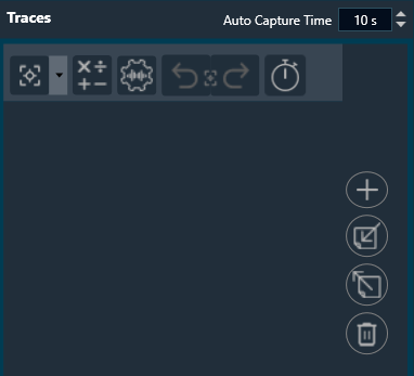
The Trace Toolbar consists of several functions.

Capture Traces

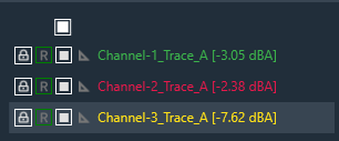
The Capture Traces function provides two options.

• Click on the button to capture all traces.
• Drop-down menu to capture individual traces.
  
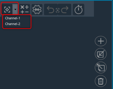
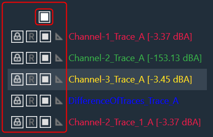
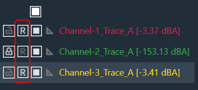
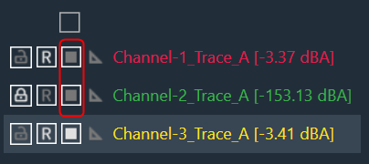
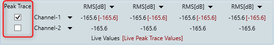
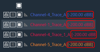
• The new captures are highlighted with a green square.
  

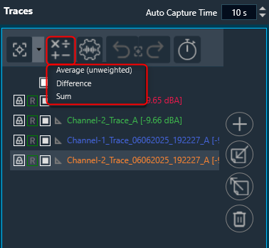
Math Operation

The Add Math Operation allows you to generate an unweighted average, a difference, or a sum trace from the selected traces using a drop-down menu, you can identify the new traces with the green square.

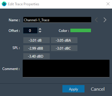
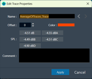
For the average math operation, if the involved traces have SPL values, the resulting average trace will also include a calculated SPL value.

• For Text Traces, the resulting average trace will have only one type of SPL value.
• For Captured Traces, the resulting average trace will include SPL values for all weightings (A, B, C, and D).
  

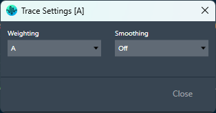
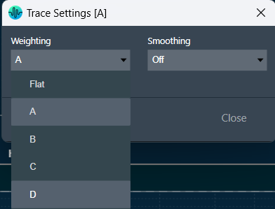
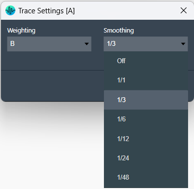
Trace Settings

The Trace Settings allow you to configure the Weighting and Smoothing functionality. For more details, refer to Trace Configuration

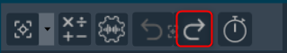
Redo and Undo Capture Traces

• Redo Capture Traces: Click on the Undo Capture Traces to reverse the last captured traces up to 3 traces.
  
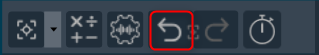
• Redo Capture Traces: Click on the Redo Capture Traces to redo the last captured traces up to 3 traces.
  

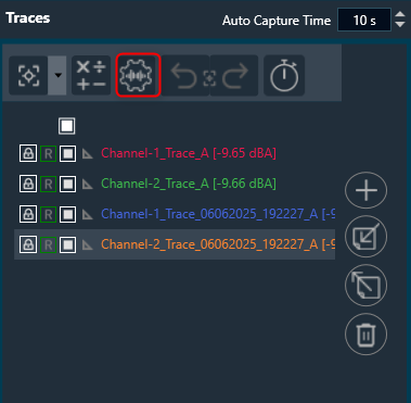
Auto Capture Traces

The traces can be auto captured by configuring the auto capture time and using the timer start and stop button.
The auto-capture time can be configured using the textbox and increment/decrement buttons in the header area.

Min value is 5s, max value is 600s, and default value is 10s.

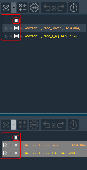
The auto capture feature supports link mode. In this case, the auto-capture in the lower graphs follows the auto-capture in the upper graph.
Auto-capture will automatically stop when the analyzer is stopped or when RTA settings are imported.
Additionally, the auto-capture time is saved in both the project file and the RTA settings file.

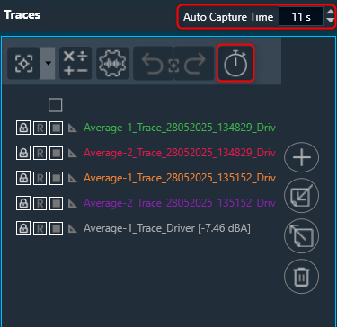
Once you have configured the time, click the “Start Timer” button. After you click this button, the timer will start, and the button will change to a “Stop” button. A countdown will be displayed over the button. You can stop the timer at any time by clicking the “Stop” button.

The traces will be captured after the configured time. The name of each automatically captured trace includes the date and time of capture.

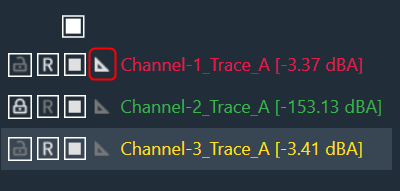
Add Target Curve

The Add Target Curve function allows you to add a target curve and edit a highlighted target curve using a drop-down menu.

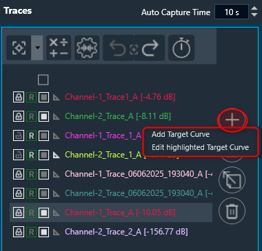
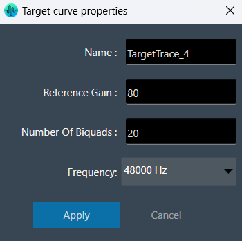
To add a target curve, click on the “Add Target Curve” option. In the target curve properties window, enter the desired curve properties, such as its name, reference gain, and number of biquads, and select the frequency for the target curve from the drop-down. Then, click “Apply” to add the target curve.

Once the target curve is active, its offset will change by 3 dB for every jump on the octave banding configuration, to follow the behavior of the energetic sum of the octave banding.

To edit the target curve, click on the “Edit Highlighted Target Curve”. In the target curve properties window, change the target curve properties and click “Apply”. This opens the Design Target Cure window, opens the Biquads on Apply to update the filters, imports, and exports the filters.
To know more about all the components on this window, refer to the Biquad Panel.

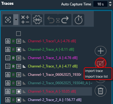
Import Traces

The Import function allows you to import single traces (*.trace) or multiple traces (*.trclist) using a drop-down menu.

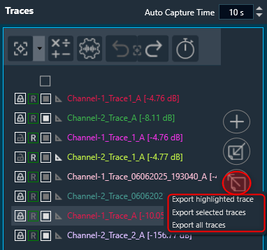
Export Traces

The Export function allows you to export the highlighted trace (*.trace, *.txt), selected traces, or all traces (*.trclist, *.trcTxtlist) using a drop-down menu. The TraceList file can be exported as a .zip file with a (*.trace, *.txt, *.trclist, *.trcTxtlist) file extension.

You can unzip the .zip file and access the individual traces from it. The exported file contains the details of the setting in the text file (sample rate, FFT size, Unit in column title, etc) used during the capture, along with the data captured.

The checked status is not retained for the tracelist exported in .txt format.

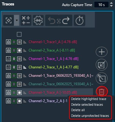
Delete Traces

The Delete function allows you to delete the highlighted trace, selected traces,  all traces, and unprotected traces using the drop-down menu.

 

The following are the operations you perform under the Trace configuration.

• Enabling Peak Hold Trace
• Setting Time Constants
• Weighting on Captured Traces
• Smoothing on Capture Traces
• Edit Trace Properties

Enabling Peak Hold Trace

The Peak Hold Trace can be activated using a checkbox in the ribbon bar – live values section. It’s time constants, Forever and Custom, can be selected in the normal Analyzer Settings in Advanced Settings window.

To activate the Peak Hold Trace, use the below option in ribbon bar,

After enabling the peak hold trace, if you switch to different channel, peak hold will be disabled on previous channel & enabled on new selected channel.

Setting Time Constants

You can configure desired time constants for the Peak Hold Trace, such as “Forever” and “Custom” in the Analyzer Settings in Advanced Settings window.

 

Weighting on Captured Traces

The A-weighting, B-weighting, C-weighting, and D-weighting are different frequency weightings that simulate how sensitive various frequencies are to the human ear.

• A-weighting (dB(A)): A-weighting is used to approximate the sensitivity of the human ear to different frequencies at low sound pressure levels. It reduces the contribution of low and high frequencies to better represent the way humans perceive sound in relatively quiet environments. A-weighted measurements are often used in assessing environmental noise levels and evaluating noise exposure limits for occupational health and safety.
• B-weighting (dB(B)): B-weighting is rarely used and has limited practical application. It was initially intended to approximate the ear’s sensitivity at moderate sound pressure levels, but it didn’t gain widespread acceptance due to certain limitations. A-weighting has largely taken the place of B-weighting in modern applications..
• C-weighting (dB(C)): C-weighting is used to measure the overall sound pressure level without any frequency weighting. It includes the entire audible frequency range and does not attenuate any specific frequencies. C-weighted measurements are commonly employed in situations where a flat frequency response is desired or when assessing high-level noise sources, such as loudspeakers or industrial machinery.
• D-weighting(dB(D)): D-weighting is used to measure sound pressure levels with a frequency weighting that is specifically designed to reflect the human ear’s sensitivity to loud noises, particularly in the presence of high-level aircraft noise. Unlike C-weighting, D-weighting emphasizes certain frequency ranges to better correlate with the subjective perception of aircraft noise.

The weighting feature is used to adjust measurements to better align with the perceived loudness by human listeners.

When you select the “Trace Settings” option in the Traces toolbar, a new window will open, allowing you to choose the desired Weighting (Flat/Unweighted, A, B, C, and D).

Based on the desired selection, weighting will be applied to all captured traces. Each trace RMS SPL value will be displayed in the traces view as shown below.

Smoothing on Captured Traces

Smoothing is a technique that reduces variations in plotted curves to improve the visual perception of trends or patterns in frequency response or level measurements. It is commonly used in audio analysis and equalization tasks to enhance clarity while considering the trade-off between noise reduction and preservation of important details.

When you select the “Trace Settings” option in the Traces toolbar, a new window will open, where you can select the desired octave banding for smoothing. Based on the desired selection, smoothing will be applied to all captured traces.

The smoothed curve with the chosen option looks like the figure below.

Edit Trace Properties

You can modify all the captured traces. Double-click on the trace to open the Trace properties window.

On the Trace properties window, you can modify the following property.

• Name of the trace – Modify the name of the trace.
• Offset value – Change the offset value.
• Color – Change the color of the trace.
• Comment – The provided comment will be exported and imported along with the trace.

In RTA, the Recorder is a sink type that allows recording in mono or stereo mode, with the option to configure the number of channels to be recorded. The Recorder supports both “Append” and “Overwrite” modes and can be synchronized with the generator signal.

To configure the Recorder settings, navigate to the Recorder tab in the RTA Settings window.

The below example shows Recorder is set to 5 channels with mono mode.

• Mono mode: 1 channel will record per file.
• Stereo mode: 2 channels will record per file. Recording can be appended to the same file or overwritten using Record mode.
• Sync with Generator: The Recorder and Generator will be in sync with this option. When the Generator starts, the recording begins automatically, and vice versa.
  Choose the generator instance from the drop-down menu that is synchronized with the recorder.
• Use Scale Offset: The scaling factor can be used to amplify or attenuate the recorded signal, as explained in the information tooltip. Scale offset can be set per recording channel.

When you click on the “Close” button, the selected file for the channel is removed from the tab settings, and the channel is closed for recording until the settings are applied with the “Done” button.

Max supported recording channels are 64 and supported recording file format is .Wav.

Once you have finished configuring the recorder, use Start or Stop the recorder and Pause or Resume it.

Before you set the “Sound In” and “Sound Out” devices, make sure you have configured sound card settings like Host API (Driver Protocol), Device, Sample Rate, and Block length of the sound card. Refer to the Sound Card Configuration to know about configuration details.

After selecting a Host API, it is necessary to choose the Sound In and Sound Out devices. If no device is selected, RTA will operate in a silent mode, which can be useful for verifying generator modes or analyzing pre-recorded measurements from a .wav file.

The stream channel pairs, labeled as Sound In 1 to 16 and Sound Out 1 to 16, are accessible in the analyzer and routing settings. You can select these channels from the context menu to establish connections between sound card channels and RTA processing blocks.

In case the device block length is higher than your sound card block length. It will introduce an additional latency in the signal chain, which will cause a shift in the start position and missing blocks at the end of the recording.

For example, if the device block length is equal to 4096 and the sound card block length is equal to 1024, there will be a “drift” of 3-blocklengths or 3072 as you can see below.

Known Issues: When importing GTT Projects older than the “W” release. If sound In and Out devices are not assigned in the soundcard setup, IVP processing will be disabled, and a pop-up message will be displayed.

To troubleshoot this issue, configure the sound In and Out and then proceed to IVP settings.

The Plugin Host is a host for virtual amp dll. The Plugin Host supports up to 3 instances of plugins (virtualAmp.dll in 64-bit), which are executed in series.

The block sizes and sample rate will be determined by the sound card settings and will be applied to all plugins. If the block size of the device/instance does not match the plugin’s block size, the plugin needs to internally handle the block size conversion.

The Virtual Amp does not support sample rate conversion in the current version. If a sample rate conversion is attempted, an error message will be displayed, and the processing will be stopped.

• Steps to Configure Plugin Host
• Connect to the device through Plugin Host

Steps to Configure Plugin Host

1. Navigate to the IVP RTA tab and select Advanced from the ribbon bar. This opens the RTA Settings dialogue box.
2. On the RTA Settings dialogue box, select the Plugins tab.
3. Click on the folder icon to browse the xAF library path.
4. Set the port number under the Port box.
5. Enable the Bypass option (optional), if you prefer the input to be passed directly to the next plugin or output without undergoing any processing.
6. Click on Apply. The number of inputs, number of outputs, and plugin type will be automatically updated based on the provided signal flow. Similarly, you can set the remaining plugins.
   Click on Reset (optional), to set back all the values in a specific row to their default values.
   
7. Go to the Routing [in] tab.
8. Set the inputs for “Plugin Host” (such as Generator1 and Generator2). These inputs will determine the channels from the Plugin Host that will be used.
9. Set inputs for “SoundOut” in order to route the PluginHost output channels to the sound card outputs.
10. If you want to display the output of PluginHost in RTA (optional), go to the Analyzer tab and select Plugin Host output as the channel source.
11. Set the Channel source (such as Generator1, Generator2, PluginHost1, and PluginHost2) to display in the chart.
    
12. Once the settings have been updated, click Done.

    By default (no flash file available next to the virtualAmp.dll), the number of in-/outputs in the plugin host is -1.

    The default Port Number starts from 25001.

Connect to the device through Plugin Host

1. Click Plugin Host.
   
   

   The Plugin host button is disabled until you select a valid plugin host.

2. Switch to the Signal Flow Designer window, configure signal flow, and click on Send Signal Flow. A pop-up message will ask you to reboot the device.
3. Switch to the IVP RTA tab and click Reboot.
   
   
4. Switch to the Device Designer tab and click on Connect Device to connect to the device.
   
5. A device synchronization dialogue box will appear, enable the desired synchronization option, and click Send.
   
   

   If AmpSrv is unable to connect, close it and retry.

   Now you can perform tuning on the IVP RTA.

6. Switch To the IVP RTA tab and click on the Generator and Analyzer option. In the graph section, the generated signal will be displayed.
   
   

7. Click on Channels to see the values of each channel. If you want to configure the graph, click on Advance Settings and go to the Graph setting.
   

Click on the “Analyzer Settings” to open the advanced RTA setting dialogue box. Here you can configure different analyzer settings.

By default, the Auto-Completion is enabled, and allows auto-filling of sources for Analyzer channels and Routings.

The following modifications can be made in the Analyzer setting window using the channels list:

• Source: This defines the input of a certain analyzer channel. By clicking on the control, a context menu pops up from which the desired source can be chosen.

  If there is no input available, “None” will be shown as the source by default.

  

• Name: Enter the name of an analyzer channel. This name appears in the channel viewer and will be set as a default name when storing measurements as traces.
• Calib[db]: When a channel is being calibrated for a certain microphone, the determined value appears here. It can also be overwritten by entering a desired value. The unit is “dBFS”; the analyzer input stream will be scaled by this value. Based on the microphone calibration unit, this unit will be set. The same unit will be suffixed to the Y-axis unit for the Spectrum mode graph. Examples: dBFS(RMS), dBSPL(RMS) etc.
• AvgCH: When the analyzer is in “Multiplexer” mode, this control determines to which “Average” channel the analyzer source is added. When the channel is “0,” it is not included; when it is “1” or “2,” it is added to “Average-1” or “Average-2,” respectively.

  Channels 17 and 18 are reserved for the “Average” channels. Here, only the name can be edited.

• Delay: Add or subtract time delay in milliseconds. In Phase measurement, we can add/subtract time delay to compensate for HW and/or acoustic delay.
• Compensate Mic:  If this flag is enabled and the analyzer source is Sound-In, its respective compensation files will be considered for magnitude curve correction.

Additional Analyzer settings

---

• FFT Settings
• Average Settings
• Live Values (RMS)
• Peak Hold
• Clipping

FFT Settings

The length of the FFT, which is used for the spectrum calculation, can be set between starting from 4096 up to 131072 samples (4k to 128k). The higher the value, the finer the frequency resolution of the spectrum. But with increasing lengths, the CPU load will increase due to the higher number of calculations and data to plot.

You can specify how a finite data set is extracted from the roughly infinite input data stream using the “FFT Window”. The “FFT Length” determines how the data set is cut out. For more details about windowing, refer to the Window Functions.
“Hann” will be the default value for the FFT window. The Weighting function allows you to select how the input signal is weighted across the frequency range. These support A, B, C, and D weightings. For more details about weighting, refer to the A-weighting.

Weighting is also available in Live values. If both weightings are selected, the weighting selected in spectrum settings is applied first, followed by the weighting selected in Live values. If you would like to monitor the live values independently of the spectrum weighting, please select the spectrum FFT Freq Weighting as Flat.

The FFT Averaging setting defines how averaging is applied to the signal, determining how spectral data is smoothed over time. RMS and FFT averaging are always linked together.

• Fast: Small averaging time constant and hence only a small amount of smoothing.
• Slow: Large averaging time constant and hence significant smoothing.
• Forever: Extreme averaging time constant.
• Custom: User-defined averaging time constant.

Average Settings

Mode Average: This setting defines how averaging is applied to the signal, determining how spectral data is smoothed over time.

• Time: In “Time” mode, the analyzer works as a multiplexer. It combines multiple input audio signals into one audio signal by dividing the input channels into equal fixed-length time slots and mixing them into a common output channel with fading between channels. The length of the time slots and the fading characteristic can be configured during runtime. The output signal is the signal of one input channel at a time. If the last input channel is reached, the next input channel will be the first input channel again. Since in this mode only one or two spectrums are calculated, it can be used when CPU load is an issue.
  Activating the multiplexer mode to “Time” allows you to set the length of a time slice (referred as “Period Time”) and the time duration for fading one channel into the next (referred to as “Fade Time”).
• Frequency (Power): Averages the power spectrum across frequency bins. Power averaging is performed in the linear domain, ensuring accurate representation of total energy distribution in the frequency spectrum.
• Frequency (dB/Linear): Averaging of decibel values treats all sounds equally, unlike power averaging, which gives more weight to louder sounds. This ensures that higher-level measurements shift the average level without significantly altering the curve’s overall shape, making it useful for analyzing relative variations without bias toward louder components.

Live Values (RMS)

Applies standardized frequency weighting to match human hearing perception. These support A, B, C, and D weightings. For more details about weighting, refer to the A-weighting.

Make sure to keep the FFT Freq Weighting as ‘Flat’ in Spectrum settings to impact only the Live Ribbon RMS values and not the graph.

Peak Hold

Peak hold trace allows the analyzer to display a secondary live trace for each channel, showing the highest amplitude values for each frequency. This feature helps to mark the highest amplitude reached at each frequency.

By default, all the peak traces will be disabled. This can be enabled using the checkbox available in the Live Values group for the selected channel.

Click “Delete” in the data context menu of the peak trace in the trace list to reset it. When a peak trace is deleted, the database also deletes the current peak trace and creates a new one.

• Custom: Sets the hold time to user-defined in milliseconds.
• Forever: Holds the peak values until the Reset button in the ribbon bar is clicked.
  

Clipping

Clipping occurs when the input signal exceeds the full-scale range of the input sound device.  The Analyzer detects clipping by checking if at least two consecutive amplitude values in the time domain exceed a threshold of +-0.999999f. If a signal is clipped, it will be indicated on the top right of the graph, as shown below.

Clipping Detection mode includes:

• Off: Disables clipping detection.
• On: Enables clipping detection.