The AudioworX Starter Kit Utility GUI Tool (SKUtilityGUI.exe) is a graphical application designed to simplify remote management of Starter Kit hardware. With an intuitive user interface, the SKUtilityGUI simplifies essential operations—such as running system diagnostics, rebooting the Raspberry Pi, resetting the AWX Amp application, and configuring audio hardware. This application is a graphical front-end for the SKUtility command-line tool (described in detail in SKUtility Tool – Command-Line Interface) and communicates over a local network using Ethernet or Wi-Fi to perform remote operations of the Starter Kit.
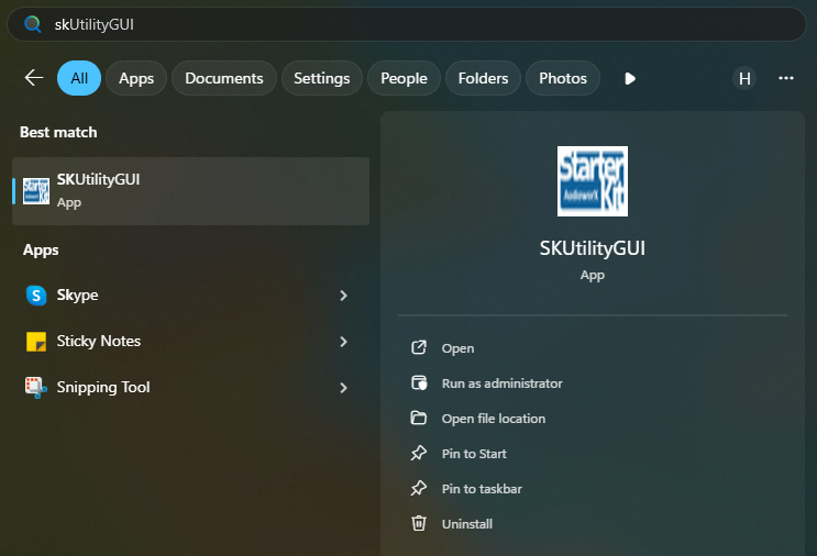
The SKUtilityGUI is installed along with GTT and can be accessed from the start-menu by pressing the “windows” key and typing “SKUtilityGUI” as shown below.
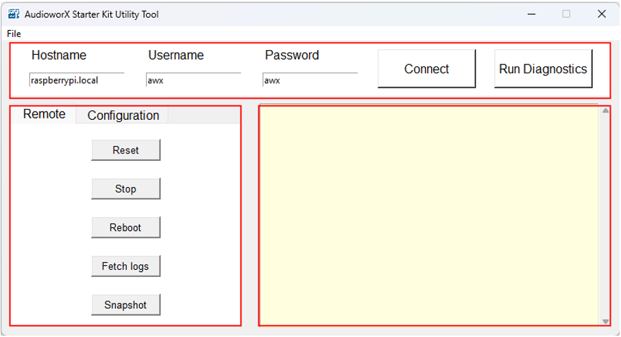
The SKUtilityGUI has the following panes:
- Login Pane (top pane): Login credentials and button for connecting remotely to the Starter Kit. Also has a button for running diagnostics.
- Function Pane (left-side pane): User functions for remotely operating the Starter Kit.
- Output Pane (right-side pane): Output log prints.
To remotely login to a Starter Kit hardware that is available on the same network as the PC, users must specify the login credentials in the login pane and click the Connect button.
The default login credentials for the Starter Kit are pre-filled. Upon changing the login credentials, the SKUtilityGUI saves the details and recalls them on subsequent launch.
The following sections explain the key functions of the SKUtilityGUI in detail.
- Running Starter Kit Diagnostics
- Starter Kit Remote Control
- Starter Kit Configuration
Running Starter Kit Diagnostics
The Run Diagnostics (right-most button on the Login pane) function runs a series of checks to verify if the Starter Kit hardware is configured and is functioning as expected. On running diagnostics, a detailed report will be generated and printed in the output pane on the right-side of the SKUtilityGUI.
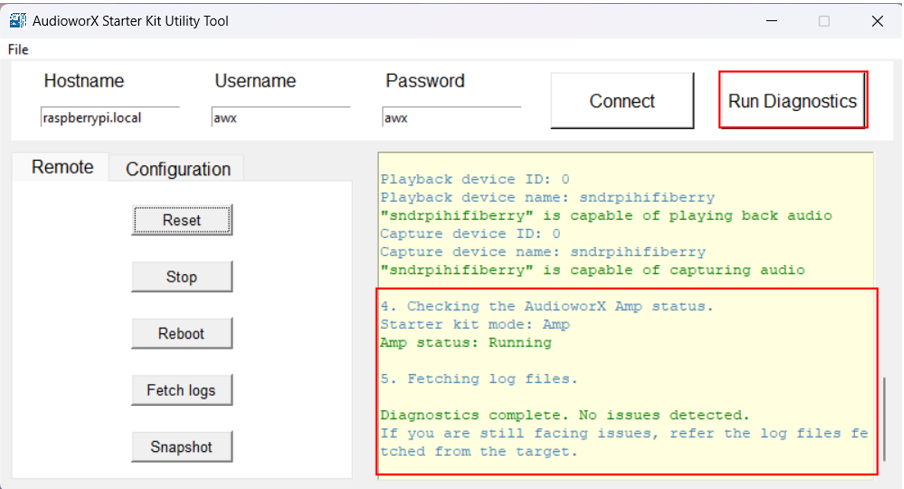
The diagnostics only identifies issues in the configurations of the hardware that may be preventing proper operation of the AWX Amp application. If the Starter Kit is not functioning properly despite the diagnostics report showing no issues, refer to the log files fetched during the diagnostics to debug. The details on debugging using the Amp log file are given in the “AWX Amp Application Logs” section of Starter Kit Troubleshooting.
The “SKUtility Diagnostics Report” section in Starter Kit Troubleshooting describes the steps in the diagnostics in detail and highlights troubleshooting steps for resolving issues detected.
The SKUtilityGUI has a tab-pane on the left-side of the window with 2 tabs, namely, Remote and Configuration. The following sections describe the functions of the two tabs in detail.
Starter Kit Remote Control
The first tab in the Function pane is the Remote tab, which provides actions pertaining to remote operations on the Starter Kit, such as rebooting the Raspberry Pi, stopping and resetting the AWX Amp application, fetching log files and taking a snapshot of the Starter Kit data files. The below figure shows a screenshot of this tab.
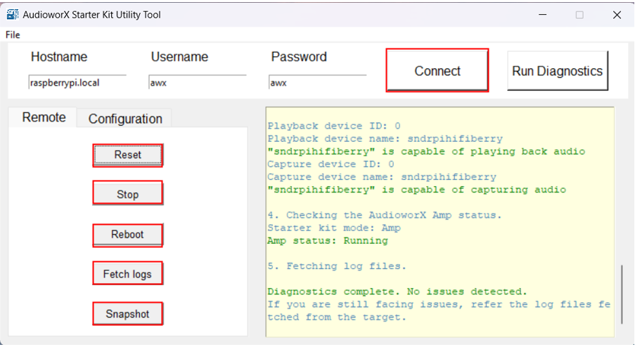
The following are the options available to a user in the Remote tab:
-
- Reset: To reset the AWX Amp application (required when updating the device definition on GTT).
- Stop: To stop the AWX Amp application.
- Reboot: To reboot the Raspberry Pi remotely. The GUI utility tool will trigger reboot and disconnect automatically. Upon reboot, the user must click the Connect button to reconnect to the Starter Kit. The reboot operation may take some time.
- Fetch Logs: To fetch the log files from target. This will open the location of the saved log files on the PC in a File Explorer window.
This will fetch two log files from the target Starter Kit hardware:
- awx_log.txt: This file contains logs related to booting up of the Starter Kit hardware and running of the AWX Amp application.
- VirtualAmpLog.txt: This file contains logs from the xAF framework that include initialization of the audio core, core AO, xAF instances, etc.,
based on the signal flow flashed on the Starter Kit hardware from GTT.
- Snapshot: To take a Snapshot of the Data Files on the Starter Kit Hardware. This will open the location of the saved snapshot file on the PC in a File Explorer window.
This function allows users to take a back-up of the Starter Kit directory in the Raspberry Pi either as a safety mechanism or to help Harman AudioworX provide debug support.
Starter Kit Configuration
The second tab in the Function pane of the SKUtilityGUI is the Configuration tab. This tab provides configuration actions for the user to modify the behavior of the Starter Kit hardware, and the audio interface connected.
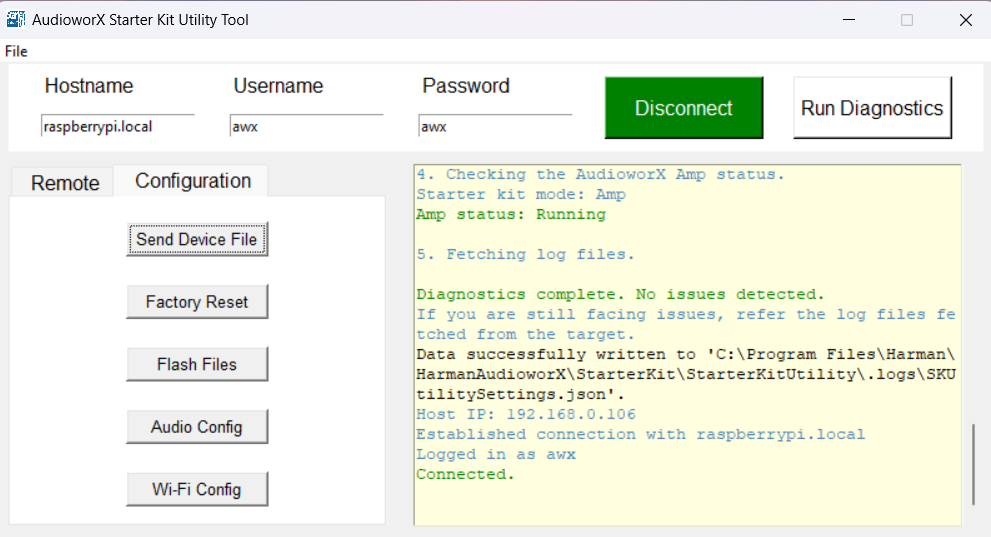
The following sections explain in detail the actions that can be performed on this tab.
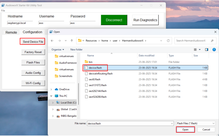
Send Device File
The “device.flash” has the necessary information about the device’s capabilities for the AWX Amp application to setup and run an audio processing pipeline. The steps for generating the “device.flash” file on GTT are illustrated in “Configuring a Custom Device Compatible with the AudioworX Starter Kit” in the “Adding a Device to the Project” section of Creating a New Project on GTT.
On clicking the Send Device Config button, a file explorer will open, prompting the user to select the device.flash file as shown below.
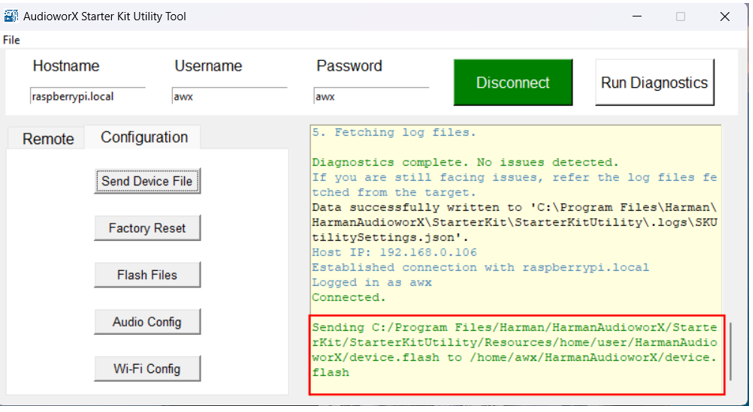
On completion of the action, a status log will be displayed in the output pane as shown below.
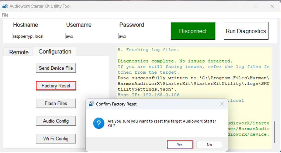
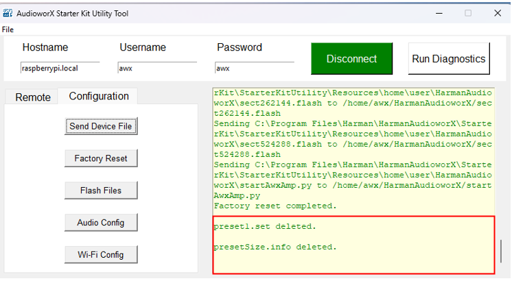
Factory Reset
This function will reset the Starter Kit hardware to its default state. On user confirmation, all files related to the AWX Amp application will be deleted from the Starter Kit hardware and restored to the default state associated with the installation of GTT.
This function can also be used to upgrade/downgrade the Starter Kit to the version of GTT installed on the PC.
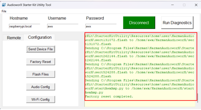
On completion of the action, a status log will be displayed in the output window as shown below.
Flash Files
The AWX Amp application uses flash files for setting up and running audio processing pipelines, which contain information about the device capabilities (audio inputs and outputs, core-type, number of virtual cores, etc.), the SFD, presets, wav files, to name a few. On flashing a new project from GTT, the flash files in the Starter Kit may need to be removed manually for smoothly setting up and running the new audio processing pipeline.
Clicking the Flash Files button opens a window that lists all the flash files that are currently present in the Starter Kit. Users may select one or more files (or all files using the Select All button) listed in the window to remove from the Starter Kit and click the Delete button to continue.
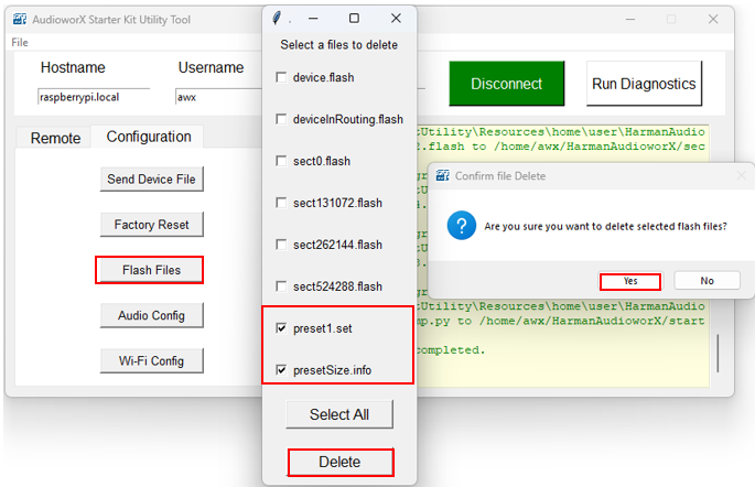
On user confirmation, the selected files will be removed from the Starter Kit (see logs in the output pane).
Audio Config
This function allows users to configure the audio device settings to be used by the AWX Amp application. By default, the Starter Kit is configured to use the HiFiBerry DAC8x and ADC8x Add-on combo as the audio interface, at 48000 Hz sample rate and 2048 sample block length.
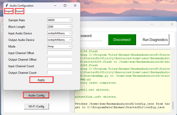
Users can configure the following:
- Sample Rate: Currently, the only supported sample rate by the AWX Amp application is 48 kHz. More sample rates will be enabled in future releases.
- Block Length: This parameter is the number of samples that the AWX Amp application will fetch and write to the audio device in one cycle. This block length is different from the block length of an Xaf Instance in the SFD, which is variable and can be configured in GTT.
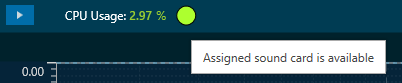
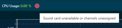
- Input Audio Device: Users can choose from one of the available (connected) audio devices for the AWX Amp application to fetch input audio samples from. Note that only audio devices that can capture audio samples will be listed.
- Output Audio Device: Users can choose from one of the available (connected) audio devices for the AWX Amp application to output audio samples. Note that only audio devices that can play back audio will be listed.
- Mode: Users can choose from one of 2 modes for the Starter Kit to boot into:
- Amp Mode – In this mode, the AWX Amp application is automatically started the Raspberry Pi boots up. Users must ensure that the selected audio devices (both input and output) are connected while powering on.
- Dev Mode – In this mode, the auto start of the AWX Amp application is disabled and is only meant for developers to debug the audio processing pipeline.
- Input Channel Offset and Output Channel Offset: These parameters are used to specify the starting index of the audio channels on the sound card that the amplifier should use. These parameters are useful when using only a sub-set of the available audio input and output channels in the audio interface. For example, when only using the back-side input ports (channels 11 to 16) and output ports (channels 3 to 8) on the TASCAM 16×8 audio interface, users can set the offsets as 11 and 3 for the input and output channels, respectively, and the AWX Amp application will only use the channels from the specified indices, up to the specified number of channels (Input and Output Channel Counts).
- Input Channel Count and Output Channel Count: These parameters are used to specify the maximum number of supported audio channels for audio input and output, respectively. While this information is typically retrieved using ALSA APIs, some audio interfaces, like the TASCAM 16×8 audio interface, do not always report the correct channel counts. In such cases, it is necessary to manually specify these values.
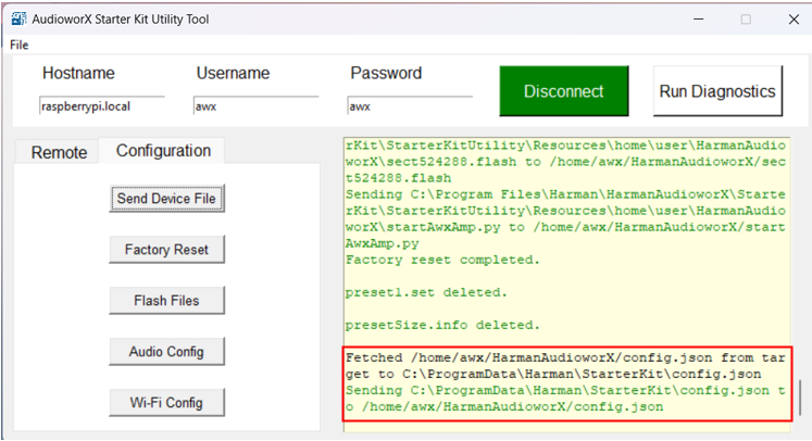
Additionally, users can save and restore audio device configurations using the Export and Import buttons on the top-ribbon bar of the Audio Config window.
Click the Apply button to send the configuration to Starter Kit (see the status message in the output pane). Once the configuration is complete, reset the AWX Amp application using Remote > Reset.
Wi-Fi Config
This function allows users to configure the wireless network settings of the Starter Kit.
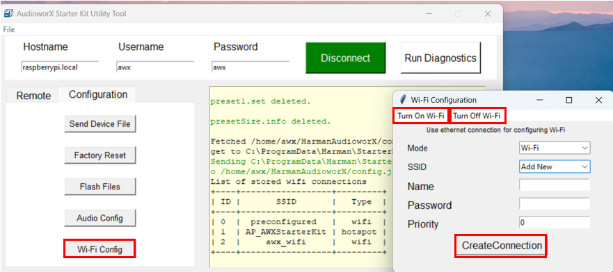
The following are the configuration options available:
- Turn On Wi-Fi: This action is used to turn on the Wi-Fi or hotspot module of the Raspberry Pi.
- Turn Off Wi-Fi: This action is used to turn off the Wi-Fi or hotspot module of the Raspberry Pi.
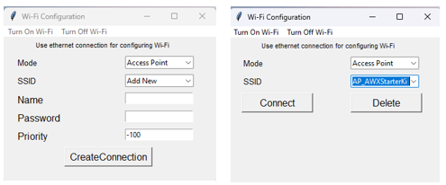
- Mode: This drop-down menu can be used to select the wireless communication mode of the Starter Kit (Wi-Fi or Access Point/Hotspot).
- SSID: This drop-down menu lists all the known Wi-Fi connections to connect to.
- To add a new connection, users can select the “Add New” option, specify the Name, Password and Priority (optional) of the connection, and click the CreateConnection button to connect to the new Wi-Fi network. The optional Priority parameter can be used to set the priority of the Wi-Fi or Access Point connection for the Starter Kit to auto-connect on boot-up (range: -999, 999, where higher the number, higher the priority). By default, the priority is set to 0 for Wi-Fi mode and -100 for Access Point (hotspot) mode.
- To connect to a known network, users can select the SSID from the drop-down menu and click the Connect button.
- To remove a known network from the list, users can select the SSID in the drop-down menu and click the Delete button.
The Starter Kit is configured by default to start up a Wi-Fi hotspot named “AP_AWXStarterKit” with the password “starterkithotspot” to enable direct wireless connection from a PC when wired connection is not possible. Users can connect to this hotspot on first-time use from a PC and reconfigure the Starter Kit using the Wi-Fi Config option in the SKUtilityGUI to connect to a different Wi-Fi network.