GTT Installation

During GTT installation, the following issues may occur. You can refer to the solutions provided.

Issues during GTT Installation
SQL Installation Issues
Issues during GTT Launch

Issues during GTT Installation

Issue	Description and Solution
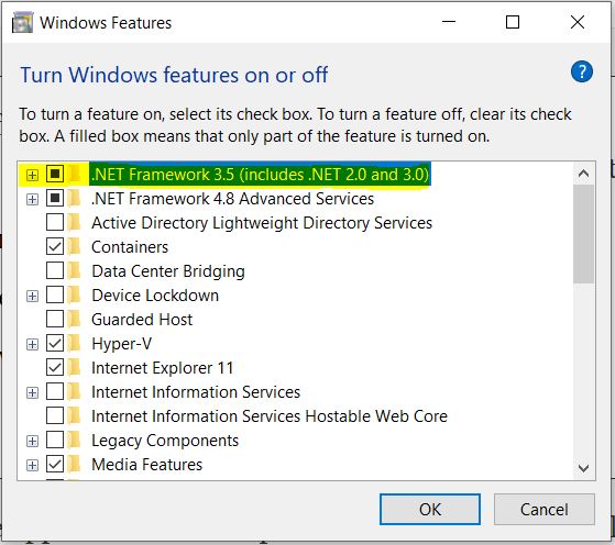
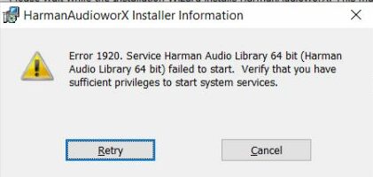
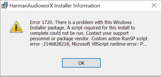
Service Installation error message	Description During installation, the following error message appears. Solution This error occurs if the default .NET 3.5 is not enabled on Windows. Check if the feature is enabled from Windows features.To do this, follow the steps below: Go to Control Panel > Programs and Features. On the left panel, select View Windows features on or off. Check if the below highlighted feature of .NET is enabled or not.
Installer Error Message	Description During installation, the error message below appears. Solution This error message appears if there are previous residues of service left. Follow the steps below: Click on Abort. Run services.msc and check if the Harman Audio Library service is in the list. If it is in the list: Run CMD (as administrator) and type sc delete “Harman Audio Library”. Same steps can be used for Harman License Manager as well.
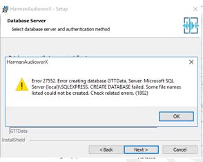
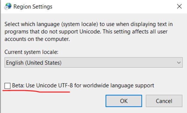
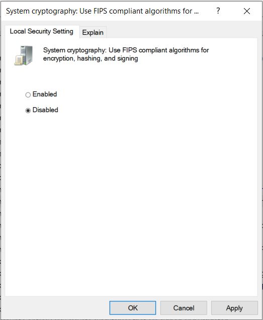
Database Error Message	Description During installation at the database selection step, getting below error. Solution Before installing GTT, navigate to this location C:\Program Files\Microsoft SQL Server\MSSQL15.SQLEXPRESS\MSSQL\DATA Check if these two files are already present. – GTTData.mdf – GTTData_log.ldf If they exist, create a backup of them and remove them from this location. Then, attempt the installation again. There are chance that the below checkbox is checked. Uncheck this. This is available in Control Panel -Time & Language > Region Settings. To reach the above option, go to Control Panel > Clock and Region > Region > Administrative tab.
Installation is failing without any specific error.	Description In some scenarios we have seen, installation fails without any error, just says “Installation interrupted.” Solution This issue mainly comes due to an issue in SQL state on the system. For example, if the SQL port is blocked or the service is in the stopped state. To resolve this, follow the steps below to write to the database: Enable TCP\IP protocol and Named Pipes from the SQL configuration manager. Restart the SQLEXPRESS service from SQL Configuration Manager. Enable TLS 1.0 protocol, to do this in RUN-> type regedit, press enter. Navigate to the key in the registry. (HKEY_LOCAL_MACHINE\SYSTEM\CurrentControlSet\Control\SecurityProviders\ SCHANNEL\Protocols\TLS 1.0) Under TLS 1.0 u will find Client and Server, for both the keys, do the settings as shown in the screenshot. Make sure to do for both the Client and the server. Restart the SQLEXPRESS service. Then try the GTT installation. Sometimes we have to repeat these steps a couple of times so that the GTT installer can write to the database.
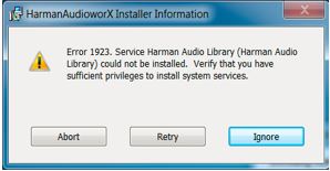
Installation error	Description During installation getting below error. Solution Before Installing, Go to C:\ProgramData\Harman\GTT folder. Check if AudioLibraries folder exist, if exists delete or rename it. Try installation again.

SQL Installation Issues

Issue	Description and Solution
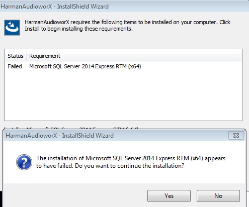
SQL Installation Fails	Description The installer complains that the SQL RTM installation has failed. Solution There seems to be another version of SQL Compact edition installed on the box. Cancel the installation by clicking “No” or click OK. Restart the machine. Try the installer setup again. Microsoft SQL RTM has a rule to check if there is any pending restart on the machine, if pending SQL installation will fail.
HarmanAudioworX installation fails	Description Sometimes the SQL Express is not installed with the pre-reqs. This may be because the system would have had the SQL Express installed previously and uninstalled, however, the registry is not cleaned properly, and the Pre-reqs wrongly detect the installation and skip. Solution Manually install the Microsoft SQL 2019 server Express edition. Link: SQL_2019
AudioworX_PreReq fails on Windows 11	Description If the machine has been upgraded from Windows 10 to Windows 11, the AudioworX_PreReq installation fails due to SQL Server Express 2019 incompatibility. Solution If the machine has been upgraded from Windows 10 to Windows 11, ensure the following registry key exists before proceeding with the SQL Server Express 2019 installation. To add the registry key, open Command Prompt as Administrator and run the following command: REG ADD “HKLM\SYSTEM\CurrentControlSet\Services\stornvme\Parameters\Device” /v “ForcedPhysicalSectorSizeInBytes” /t REG_MULTI_SZ /d “ 4095” /f* Once you have added the registry key, run Setup_HarmanAudioworX_PreReq_2.2.0.2450.exe.

Issues during GTT Launch

Issue

Description and Solution

GTT Launch

Description

When you are trying to launch GTT from a different account (which was not used for installing GTT).

Solution

This is not a valid scenario as it has not been fully tested. Hence, we recommend using the same account that was used for installing GTT to launch GTT.

March 25, 2025

AmpSRV2

Issue Title

Description

Potential Solution

AmpSrv2 disconnected from GTT

Disconnection can have several sources:

GTT request disconnect
Disconnect is requested by AmpSrv2 GUI / pressing ESC: Then you should get a message box like:


AmpSrv2 Disconnection

The socket connection between GTT and AmpSrv2 breaks, maybe cause by huge CPU load
AmpSrv2 detects an issue with RS232 interface. Are you using USB to serial converter? Did you checked with a different converter?

Check whether GTT requests the disconnection by doing the following:

Start attached application in parallel to your test automation.
Choose corresponding interface inside of the tool and connect to AmpSrv2.

AmpSrv2 Troubleshooting

If GTT disconnects, AmpSrv2 should still be connected to the target device.

March 25, 2025

Issue Title	Description	Potential Solution
GTT Crashes while launching streaming window.	Performance counters cannot be accessed while starting streaming.	One of the reason, GTT may crash while starting streaming could be the Performance Counters are not properly initialized or they are corrupted. This could be solved by rebuilding the performance counters. To rebuild all Performance counters including extensible and third-party counters, type the following commands at an Administrative command prompt. Press ENTER after each command. Rebuilding the counters: cd c:\windows\system32 lodctr /R cd c:\windows\sysWOW64 lodctr /R Resyncing the counters with Windows Management Instrumentation (WMI): WINMGMT.EXE /RESYNCPERF Reference: https://support.microsoft.com/en-in/help/2554336/how-to-manually-rebuild-performance-counters-for-windows-server-2008-6
Streaming Viewer stops when Laptop is removed from docking station
Workaround for LUT parameter sets unit problem[Backward compatibility]	This issue will happen with every single LUT object in every set group with this device file. What seems to happen is the panel is appending the unit of each parameter into the set file, which is corrupting it.	This workaround required for projects which are exported earlier than N+1 release. Import earlier exported project. Open Signal Flow designer , if all LUT objects belong to same group, launch panel by double clicking any LUT object. If each LUT objects belongs to different groups. Launch panels separately for each group. Close opened LUT panels. Open Parameter sets view , right click on column header of red color highlighted set and click ‘Store’ context menu to get latest set values. You can observe red highlights are cleared and units are removed for each state variable.
Unable to import/export projects in GTT	If the FIPS Algorithm Policy is enabled in the computer, GTT fails to import/export any project.	Close the GTT. Navigate to the Windows start bar and in the search field enter “secpol.msc”. This action opens the Local Security Policy editor. Under the Security Settings, navigate to Security Options, and locate the System cryptography setting. If the System cryptography setting is enabled, proceed to the next step to disable it. Double-click on the System Cryptography setting, choose Disabled, and then Apply. Reboot the computer. Launch the GTT and try to import/export any project.
Chart Rendering issue	If any issues related to Chart rendering in RTA or Streaming window.	Please update GPU/ Video card drivers to latest version. One issue found in Dell system Latitude 5420 and solved with below steps: Open URL https://www.dell.com/support/home/en-us/product-support/product/latitude-5420-laptop/drivers Download new Video card driver Intel UHD/Iris Xe Graphics Driver -> Intel-UHD-Iris-Xe-Graphics-Driver_RGVN2_WIN64_31.0.101.3959_A12.EXE from above link. Install the driver.

Enabling Streaming Functionality

Now, if you want to measure the audio signal output and control output of an audio object of the added device. You need to configure Streaming functionality in a signal flow design.

Go to the Device Designer window and select the virtual core of the device.
Go to the virtual core properties and select the Streaming checkbox to enable streaming functionality.
Enter the desired number of Level Meters that need to be added to the signal flow to monitor control-out connections or audio.
Click Save to save the changes and click on Send Device Config.
Double-click on the Xaf Instance to open the Signal Flow Designer window.
On the Signal Flow Designer window, right-click on the audio connections, and select Level Meter > RMS. This action adds Level Meters in the signal flow design.
Open Preset Controllers, click on Add Slot, and set Group 1 as LFHighOnly.
Similarly, add another slot and set Group 1 as AllSpeakers.
Click on Send to Device. When the preset data has been successfully sent, a completion message is displayed to indicate that the transmission was successful.
If an error occurs, an error message is displayed.
Click on Load Slot. The GTT sends a slot load request to the device and waits for a response.
If the device is successfully loaded into the slot, a success message is displayed on the screen. Now you can perform tuning.
Double-click on the audio object to open the native panel. On the native panel, change the value using the slider and check the level meter value.
Similarly, open the IVP RTA window, go to the native panel, change the value using the slider, and check the signal graph.

June 25, 2025

In Global Tuning Tool you can perform basic tuning using Integrated Virtual Process (IVP). In the Integrated Virtual Process (IVP) allows you to make adjustments to various aspects of the audio configuration in the signal flow designer, such as audio object mapping, parameter settings, and virtual core configurations.

For more details, you can refer video explaining basic tuning process using IVP in Global Tuning Tool.

Steps to performing basic tuning with Integrated Virtual Process (IVP)

Launch the Global Tuning Tool application.
Navigate to the Sample Project tab and click on the AWXExampleProject.

This will open the Device Designer window and display example project details.
This example project contains a single win64 core with one instance of audio processing (xAF Instance). It has 2 inputs and 8 outputs.
Double-click on the Xaf Instance to open the Signal Flow Designer window.
Navigate to the IVP RTA tab to configure the device file and input/output settings.
On the IVP RTA tab, click on Advanced Settings, under the Plugins tab, browse the xAFVirtualAmp64.dll file available in C:Program FilesHarmanHarmanAudioworXAudioFrameworkDLLs folder, and click Apply to save the plugin configuration.
Go to the Device Designer tab, click on Export > Device Template, and save the device configuration as a “.flash” file in the C:Program FilesHarmanHarmanAudioworXAudioFrameworkDLLs folder.
This will save the layout of the device (single core with 2 inputs and 8 outputs) which helps the virtual amplifier to configure itself.
Click on Send Device Config to send the changes to the device. Due to these changes, the device will go offline.
GTT will display a message “Device will go Offline. Manual Reboot of the device is required”.
Go to the IVP RTA tab and click on Reboot. Once the device is rebooted, GTT will display the message “Plugin Host has been rebooted”.Now you need to configure the input and output settings.
Open the Advanced Settings, go to the Routing tab, and under plugin host set Generator1 as input 1 and Generator2 as input 2.
Similarly, go to the Analyzer tab, under source set Generator1 as input and PlugingHost1 as output, and click Apply to save the settings.
The above settings indicate that you are using the Generator as input to the signal flow and output is displayed on the analyzer. You can also use sound card input by selecting “SoundIn1 or SoundIn2”.
Similarly, you can route the output to the sound card by choosing the Sound Out to PluginHost.
Click on Done to close the Advanced Settings window.
Click on the Design tab and click on Connect Device. This will open the Device Synchronization dialogue box.
On the Device Synchronization dialogue box, click on Send. Sending or receiving data is indicated by a progress window along with a percentage of completion of sending or receiving data. The progress bar will close automatically once the send / receive process is completed. The progress bar window title will be “Sending data” or “Receiving data” depending on your selected functionality.
Go to RTA, click on Generator, Analyzer, and PluginHost to generate input and output signals.
On the graph, the first section displays the 1^st channel of the input signal from the generator, and the second section displays the 1^st channel of output from the signal flow. You can choose to display multiple channels by configuring the Analyzer in IVP.

July 2, 2025

SKUtility Developer Options

This page contains information relevant to the developer features of the AudioworX Starter Kit, which require a special license. Write to AudioworXSupport@harman.com for details on how to avail the license.

The Starter Kit Utility (SKUtility) includes options for developers to build, flash, run and debug the AWX Amp application on the Starter Kit hardware. Following is the help text for the developer options:
python3 SKUtility.py dev -h

A screenshot of a computer program Description automatically generated — *SKUtility developer options help text*

Following are the developer actions that can be executed using the SKUtility Tool:

Developer Function	Command
Build the AWX Amp application (rpiVirtualAmp)	To build the AWX Amp application with the modified AWX External Object, run the command: `python3 SKUtility.py dev -pr rpiVirtualAmp -b`
Build the DSP library (VirtualAmp.dll) for GTT	To build the DSP library to be used in GTT with the modified AWX External Object, run the command: `python3 SKUtility.py dev -pr virtualAmp -b`
Clean the build directory	To remove traces of previous builds of either the AWX Amp application or the DSP library in the build directory, run the command: `python3 SKUtility.py dev -pr <rpiVirtualAmp/virtualAmp> -c`
Flash the AWX Amp application	To flash the custom AWX Amp application (built with the modified AWX External Object) on the Starter Kit hardware, run the command: `python3 SKUtility.py dev -pr rpiVirtualAmp -f`
Start the AWX Amp application	To start the newly flashed AWX Amp application, run the command: `python3 SKUtility.py dev -pr rpiVirtualAmp -r`Alternatively, the following command can be used to reset the AWX Amp application on the Starter Kit hardware: `python3 SKUtility.py rmt -rst`

July 4, 2025

Build AWX External Object

The GTT installation includes the source code for an example audio object called the “AWXAudioObjExt” in the following directory:

C:\Program Files\Harman\HarmanAudioworX\ext-reference-algorithms\external

It is accompanied by an audio object specification document named “AwxAudioObjExt.pdf” in the “docs” directory, explaining how the AO interacts with Extendable Audio Framework (xAF) API to implement a simple gain object.

The files “inc\AwxAudioObjExt\AwxAudioObjExt.h” and “src\AwxAudioObjExt\generic\AwxAudioObjExt.cpp” implement a class named “CAwxAudioObjExt”, which contain the functions that are called by the audio framework during initialization, tuning and run-time:

init(): Called during initialization of the SFD. Assigns memory records and sets up initial states for the AO.
calc(): Called at runtime with input and output stream buffers. Receives audio input frames from the framework and returns processed output audio frames in real-time.
tuneXTP(): Called by a parallel tuning thread to change tuning states of the AO.

These functions can be modified as required to implement a custom audio processing algorithm.

Further information can be found APIs Basic Features and APIs.

C:\Program Files\Harman\HarmanAudioworX\ext‑reference‑algorithms\external\docs\AwxAudioObjExt\AwxAudioObjExt.pdf

The custom AO source code must then be compiled and built into the DSP library for GTT and the AWX Amp application for the Starter Kit hardware, both of which can be executed using the SKUtility tool. The following sections provide instructions on building the custom dll and executable for using the custom AWX External Object.

Building DSP Library with Custom Audio Object

The “ext-reference-algorithms” directory in the installation folder contains build configuration files to build the AWX External Object. Since the modifications are assumed to be made within the existing source code, the custom DSP library for GTT file can be built directly without any updates to the build configuration files by running the following commands in the “StarterKitUtility” directory of the installation folder:

python3 SKUtility.py dev -pr virtualAmp -c # clean the build directory

python3 SKUtility.py dev -pr virtualAmp -b # build the VirtualAmp.dll file

Upon successful compilation of the code, the output DSP library dll can be found in the following location in the installation folder.

xAF\public\lib\win64\Release\VirtualAmpExternal.dll

However, if there are additional files to be compiled along with the AWX External Object source files, they must be included in the below CMake file.

ext-reference-algorithms\external\src\AwxAudioObjExt\CMakeLists.txt

Loading the Custom DSP Library in GTT

The DSP library provides a toolbox of AOs for use in a signal flow, with information on configurations and tuning parameters and their memory requirements on different core types. To be able to use the custom AO in an SFD, the custom-built DSP library must be imported into GTT.

First, start a new instance of GTT in “administrator” mode from the start menu, by right-clicking GTT and clicking Run As Administrator.
In the home screen of GTT, go to the “Audio Library Manager’ and click the Load Audio Library button.
Select the newly built “VirtualAmpExternal.dll” and click Open.

GTT may show a warning if the imported DSP library has the same version number as an existing one in the library manager. It is recommended that a backup of any previously loaded DSP library is taken for safety. The default DSP library can still be found in the “AudioFrameworkDLLs” of the installation directory.
Once the new DSP library is loaded, the custom AWX External Object can be accessed from the “Toolbox” panel under “External” tab in the signal flow designer view.

Building AWX Amp Application with the Custom Audio Object

The GTT installation also includes the necessary files to build the AWX Amp application along with the custom AO in “StarterKitrpiamp” directory of the installation folder.
To build the custom AWX Amp application, run the following commands from the “StarterKitUtility” folder.

python3 SKUtility.py dev -pr rpiVirtualAmp -c

python3 SKUtility.py dev -pr rpiVirtualAmp -b

A screen shot of a computer program

On successful completion, the “rpiVirtualAmp” executable can be found in the below location.

StarterKit\public\bin\arm64‑v8a\Release\rpiVirtualAmp

Flash the custom AWX Amp application on to the Starter Kit hardware by running the command:

python3 SKUtility.py dev -f

To start the AWX Amp application in the Starter Kit, run the command:

python3 SKUtility.py dev -r

July 28, 2025

Running Debug Session

The AudioworX Starter Kit facilitates remote debugging of custom Audio object code on the hardware with VS Code using a VS Code workspace and debug configurations that are included in the GTT installation.

Running a remote debug session requires some essential Linux packages to be present on the Raspberry Pi, which are pre-installed in the custom Raspberry Pi image. When using the official Raspbian OS, these packages can be installed using the SKUtility tool by running the command.

python3 SKUtility.py dev -stp

The Raspberry Pi must be connected to the internet to install the required packages.

Running a Debug Session for the Custom AWX External Object

The below steps illustrate how to start a remote debug session and step-through the source code of the custom AWX External Object in an SFD on the Starter Kit hardware.

First, set the Starter Kit to developer mode using the interactive configuration as explained in Starter Kit Utility Tool.
Build the AWX Amp application in “debug” mode, flash it on to the Starter Kit, and start the AWX Amp application on the Starter Kit hardware by running the following commands.
python3 SKUtility.py dev -pr rpiVirtualAmp -b -d
python3 SKUtility.py dev -pr rpiVirtualAmp -f -d
python3 SKUtility.py dev -r
Now, in the GTT window, include the AWX External Object from the toolbox into the SFD, save the SFD and click “Send Device Config” from the “Device Designer” tab of GTT to flash the SFD on to the Starter Kit.
Open a new window of VS Code, go to File > Open Workspace from File, and select the VS Code workspace file named “StartKitDebug.code-workspace” in “StarterKit” directory of the installation directory.
Open the AWX External Object source file “external\src\AwxAudioObjExt\generic\AwxAudioObjExt.cpp” from the file tree.
Place breakpoints in the source code by clicking to the left of the line number intended as shown below (line 42):
Press the “F5” key to start the debug session. This step makes use of the following files to first start a “gdbserver” on the Starter Kit hardware, and thstarts a debug session on VS Code that attaches to the remote gdbserver.

StarterKit\StarterKitUtility\.vscode\launch.json

StarterKit\StarterKitUtility\.vscode\tasks.json

Once the debug session has started, the code will stop at the placed breakpoints as shown below.
A screenshot of a computer

December 14, 2024

Reporting Issues

For reporting issues related to the AWX Starter Kit, write to AudioworXSupport@harman.com with the following information:

Subject line — “AWX Starter Kit – short description of the issue faced”
Detailed description of the issue.
Attach the following files (if any).
1. The GTT project file (.gttd) used, which can be exported from GTT (File > Export Project).
2. Snapshot of the flash files on the Starter Kit hardware which can be generated using the command python3 SKUtility.py rmt -snp. The snapshot will be downloaded to “C:ProgramDataHarmanStarterKit”.
Steps for reproducing the issue.

July 4, 2025

Overview

The AudioworX Starter Kit is intended as a simple and quick-setup tool to fully experience the design and development workflows of audio processing pipelines with AudioworX. It is comprised of commonly available hardware components to ease their sourcing across geographical locations and enable simple assembly, interfacing and usage world-over. Although the Starter Kit is still only available to users in its fully-packaged form on request (write to AudioworXSupport@harman.com), the Starter Kit is designed in a modular fashion to enable interested users even with little to no embedded-system experience to source the hardware components on their own, interface the components and configure the software to prepare the Starter Kit.

The Starter Kit also caters to more advanced users like audio DSP and algorithm engineers with developer options* enabling users to create custom audio objects for use in the AudioworX framework. The software package of the Starter Kit includes the source code for an example custom audio object, and VS Code workspace files for debugging. Additionally, the Starter Kit Utility Tool (SKUtility) is also built with developer options to streamline development and testing.

*The developer features of the AudioworX Starter Kit require a special license. Write to AudioworXSupport@harman.com for details on how to avail the license.

This document provides instructions on assembling a Starter Kit from scratch, setting up the developer environment for building and testing custom Audio Objects, building the custom executable to be run on the Starter Kit hardware, and finally running a debug session to step-through code remotely on the Starter Kit.

Related Topics

Author: Debanka