Author: Debanka

Before you set the “Sound In” and “Sound Out” devices, make sure you have configured sound card settings like Host API (Driver Protocol), Device, Sample Rate, and Block length of the sound card. Refer to the Sound Card Configuration to know about configuration details.

After selecting a Host API, it is necessary to choose the Sound In and Sound Out devices. If no device is selected, RTA will operate in a silent mode, which can be useful for verifying generator modes or analyzing pre-recorded measurements from a .wav file.

The stream channel pairs, labeled as Sound In 1 to 16 and Sound Out 1 to 16, are accessible in the analyzer and routing settings. You can select these channels from the context menu to establish connections between sound card channels and RTA processing blocks.

In case the device block length is higher than your sound card block length. It will introduce an additional latency in the signal chain, which will cause a shift in the start position and missing blocks at the end of the recording.

For example, if the device block length is equal to 4096 and the sound card block length is equal to 1024, there will be a “drift” of 3-blocklengths or 3072 as you can see below.

Known Issues: When importing GTT Projects older than the “W” release. If sound In and Out devices are not assigned in the soundcard setup, IVP processing will be disabled, and a pop-up message will be displayed.

To troubleshoot this issue, configure the sound In and Out and then proceed to IVP settings.

In RTA, the Recorder is a sink type that allows recording in mono or stereo mode, with the option to configure the number of channels to be recorded. The Recorder supports both “Append” and “Overwrite” modes and can be synchronized with the generator signal.

To configure the Recorder settings, navigate to the Recorder tab in the RTA Settings window.

The below example shows Recorder is set to 5 channels with mono mode.

• Mono mode: 1 channel will record per file.
• Stereo mode: 2 channels will record per file. Recording can be appended to the same file or overwritten using Record mode.
• Sync with Generator: The Recorder and Generator will be in sync with this option. When the Generator starts, the recording begins automatically, and vice versa.
  Choose the generator instance from the drop-down menu that is synchronized with the recorder.
• Use Scale Offset: The scaling factor can be used to amplify or attenuate the recorded signal, as explained in the information tooltip. Scale offset can be set per recording channel.

When you click on the “Close” button, the selected file for the channel is removed from the tab settings, and the channel is closed for recording until the settings are applied with the “Done” button.

Max supported recording channels are 64 and supported recording file format is .Wav.

Once you have finished configuring the recorder, use Start or Stop the recorder and Pause or Resume it.

The following are the operations you perform under the Trace configuration.

• Enabling Peak Hold Trace
• Setting Time Constants
• Weighting on Captured Traces
• Smoothing on Capture Traces
• Edit Trace Properties

Enabling Peak Hold Trace

The Peak Hold Trace can be activated using a checkbox in the ribbon bar – live values section. It’s time constants, Forever and Custom, can be selected in the normal Analyzer Settings in Advanced Settings window.

To activate the Peak Hold Trace, use the below option in ribbon bar,

After enabling the peak hold trace, if you switch to different channel, peak hold will be disabled on previous channel & enabled on new selected channel.

Setting Time Constants

You can configure desired time constants for the Peak Hold Trace, such as “Forever” and “Custom” in the Analyzer Settings in Advanced Settings window.

 

Weighting on Captured Traces

The A-weighting, B-weighting, C-weighting, and D-weighting are different frequency weightings that simulate how sensitive various frequencies are to the human ear.

• A-weighting (dB(A)): A-weighting is used to approximate the sensitivity of the human ear to different frequencies at low sound pressure levels. It reduces the contribution of low and high frequencies to better represent the way humans perceive sound in relatively quiet environments. A-weighted measurements are often used in assessing environmental noise levels and evaluating noise exposure limits for occupational health and safety.
• B-weighting (dB(B)): B-weighting is rarely used and has limited practical application. It was initially intended to approximate the ear’s sensitivity at moderate sound pressure levels, but it didn’t gain widespread acceptance due to certain limitations. A-weighting has largely taken the place of B-weighting in modern applications..
• C-weighting (dB(C)): C-weighting is used to measure the overall sound pressure level without any frequency weighting. It includes the entire audible frequency range and does not attenuate any specific frequencies. C-weighted measurements are commonly employed in situations where a flat frequency response is desired or when assessing high-level noise sources, such as loudspeakers or industrial machinery.
• D-weighting(dB(D)): D-weighting is used to measure sound pressure levels with a frequency weighting that is specifically designed to reflect the human ear’s sensitivity to loud noises, particularly in the presence of high-level aircraft noise. Unlike C-weighting, D-weighting emphasizes certain frequency ranges to better correlate with the subjective perception of aircraft noise.

The weighting feature is used to adjust measurements to better align with the perceived loudness by human listeners.

When you select the “Trace Settings” option in the Traces toolbar, a new window will open, allowing you to choose the desired Weighting (Flat/Unweighted, A, B, C, and D).

Based on the desired selection, weighting will be applied to all captured traces. Each trace RMS SPL value will be displayed in the traces view as shown below.

Smoothing on Captured Traces

Smoothing is a technique that reduces variations in plotted curves to improve the visual perception of trends or patterns in frequency response or level measurements. It is commonly used in audio analysis and equalization tasks to enhance clarity while considering the trade-off between noise reduction and preservation of important details.

When you select the “Trace Settings” option in the Traces toolbar, a new window will open, where you can select the desired octave banding for smoothing. Based on the desired selection, smoothing will be applied to all captured traces.

The smoothed curve with the chosen option looks like the figure below.

Edit Trace Properties

You can modify all the captured traces. Double-click on the trace to open the Trace properties window.

On the Trace properties window, you can modify the following property.

• Name of the trace – Modify the name of the trace.
• Offset value – Change the offset value.
• Color – Change the color of the trace.
• Comment – The provided comment will be exported and imported along with the trace.

The Trace Toolbar consists of several functions.

Capture Traces

The Capture Traces function provides two options.

• Click on the button to capture all traces.
• Drop-down menu to capture individual traces.
  
• The new captures are highlighted with a green square.
  

Math Operation

The Add Math Operation allows you to generate an unweighted average, a difference, or a sum trace from the selected traces using a drop-down menu, you can identify the new traces with the green square.

For the average math operation, if the involved traces have SPL values, the resulting average trace will also include a calculated SPL value.

• For Text Traces, the resulting average trace will have only one type of SPL value.
• For Captured Traces, the resulting average trace will include SPL values for all weightings (A, B, C, and D).
  

Trace Settings

The Trace Settings allow you to configure the Weighting and Smoothing functionality. For more details, refer to Trace Configuration

Redo and Undo Capture Traces

• Redo Capture Traces: Click on the Undo Capture Traces to reverse the last captured traces up to 3 traces.
  
• Redo Capture Traces: Click on the Redo Capture Traces to redo the last captured traces up to 3 traces.
  

Auto Capture Traces

The traces can be auto captured by configuring the auto capture time and using the timer start and stop button.
The auto-capture time can be configured using the textbox and increment/decrement buttons in the header area.

Min value is 5s, max value is 600s, and default value is 10s.

The auto capture feature supports link mode. In this case, the auto-capture in the lower graphs follows the auto-capture in the upper graph.
Auto-capture will automatically stop when the analyzer is stopped or when RTA settings are imported.
Additionally, the auto-capture time is saved in both the project file and the RTA settings file.

Once you have configured the time, click the “Start Timer” button. After you click this button, the timer will start, and the button will change to a “Stop” button. A countdown will be displayed over the button. You can stop the timer at any time by clicking the “Stop” button.

The traces will be captured after the configured time. The name of each automatically captured trace includes the date and time of capture.

Add Target Curve

The Add Target Curve function allows you to add a target curve and edit a highlighted target curve using a drop-down menu.

To add a target curve, click on the “Add Target Curve” option. In the target curve properties window, enter the desired curve properties, such as its name, reference gain, and number of biquads, and select the frequency for the target curve from the drop-down. Then, click “Apply” to add the target curve.

Once the target curve is active, its offset will change by 3 dB for every jump on the octave banding configuration, to follow the behavior of the energetic sum of the octave banding.

To edit the target curve, click on the “Edit Highlighted Target Curve”. In the target curve properties window, change the target curve properties and click “Apply”. This opens the Design Target Cure window, opens the Biquads on Apply to update the filters, imports, and exports the filters.
To know more about all the components on this window, refer to the Biquad Panel.

Import Traces

The Import function allows you to import single traces (*.trace) or multiple traces (*.trclist) using a drop-down menu.

Export Traces

The Export function allows you to export the highlighted trace (*.trace, *.txt), selected traces, or all traces (*.trclist, *.trcTxtlist) using a drop-down menu. The TraceList file can be exported as a .zip file with a (*.trace, *.txt, *.trclist, *.trcTxtlist) file extension.

You can unzip the .zip file and access the individual traces from it. The exported file contains the details of the setting in the text file (sample rate, FFT size, Unit in column title, etc) used during the capture, along with the data captured.

The checked status is not retained for the tracelist exported in .txt format.

Delete Traces

The Delete function allows you to delete the highlighted trace, selected traces,  all traces, and unprotected traces using the drop-down menu.

 

Saving RTA Settings

Once you complete all the RTA settings, click on the “Save” option. A file save dialog box will appear, enter the file name, and click Save.

Upon clicking “Save” within the dialog box, all of the following settings will be exported to a file with the. rta extension in a human-readable JSON format.

• Generator
• Analyzer
• Audio Driver
• Display

Loading RTA File

Upon clicking the “Load” button, a file open dialog box will be displayed. Locate the desired .rta file and click “Open” to restore the RTA settings stored in that file. The loaded settings will take effect immediately.

If the sound card settings are invalid when you load the settings, a settings window will be launched. You will need to fix the sound card settings issue before being able to proceed further.

Upon clicking the “Apply” button, the sound card settings will be applied. Subsequently, you can modify other settings according to your preferences.

After importing the settings, it is necessary to reconnect the device.

Audio signal routing refers to the process of directing audio signals from a source to one or multiple destinations within an audio system. In audio systems, signal routing can be achieved through different methods, depending on the complexity and requirements of the setup.

On the Routing tab, the connections to the sound-out devices, plugin host, mimo convolved, and file recorder can be set.

The Sound Out channels 1 to 16 correspond to the channel pairs found in the “Streams” section of the “Sound Card” settings. Click on a control in the “Sound Out” column brings up a context menu from which you can choose a source.

Currently, the player is not supported as a source.

The Analyzer channels (excluding Average channels) can be set as a source for the recorder to any Routing sinks. The recorded data should be the same as the analyzer data if the Analyzer is set as the source for the recorder.

Upon clicking “Routing Preview,” a use case overview will appear to enhance the understanding of Routing.

Convolution is the process of multiplying the frequency spectra of our two audio sources: the input signal and the impulse response. By doing this, frequencies that are shared between the two sources will be accentuated, while frequencies that are not shared will be attenuated.

This phenomenon occurs when the input signal adopts the sonic characteristics of the impulse response, resulting in enhanced frequencies that are commonly present in both the impulse response and the input signal.

Steps to configure MIMO Convolver

1. Navigate to the IVP RTA tab and select Advanced from the ribbon bar. This opens the RTA Settings dialogue box.
2. On the RTA Settings dialogue box, select the Plugins tab.
3. Click on the folder icon to browse the xAF library path.
4. Set the port number under the Port box.
5. Enable the Bypass option (optional), if you prefer the input to be passed directly to the next plugin or output without undergoing any processing.
6. Click on Apply. The number of inputs, number of outputs, and plugin type will be automatically updated based on the provided signal flow.
7. Switch to the MIMO Convolver tab.
8. Set the number of Inputs, Outputs, and Filter Taps.
   

You can configure coefficients in 2 ways.

• Configure coefficients in Panel
• Configure coefficients through virtual prediction

Configure coefficients in the Panel

1. On the MIMO Convolver tab, click on Configure Coefficients. The Configure Coefficients panel launches with 2×2 filters.
   
2. Adjust the coefficients by either setting them to a flat value or importing them using CSV/XML files.
3. Click on Tune, after assigning coefficients.

A toast message “Tuning applied” appears.

Amplitude/Phase: When the coefficients are given and the “Amplitude/Phase” option is selected, the graph displays the value.

Coefficients:  When the coefficients are given and the “Coefficients” option is selected, the graph displays the values as per the below figure. You can change the graph style using the “Chart Style” option.

Line chart style: when “Chart Style” is selected as Line, the Coefficients graph.
Dot chart style: when “Chart Style” is selected as Dot, the Coefficients graph.

Group Delay: When the coefficients are given and the “Group Delay” option is selected, the graph displays the values.

Curves Legend: This option allows you to show the details of which graph tab (Amplitude/Phase, Coefficients, Group Delay) is selected.

On the selection of the Amplitude/Phase graph tab Curves Legend will show the below information.
On the selection of the Coefficients graph tab and Chart Styles ‘Dots’, Curves Legend will show the below information.
On the selection of the Coefficients graph tab and Chart Styles ‘Line’, Curves Legend will show information.
On the selection of the Group Delay graph tab, Curves Legend will show information.

Additional Functionalities

• Flat: This is used to make the graph flat by making coefficients to 0.
• Import: This function is used to import the coefficients for a single active filter. Click on the “Import” button, then enter the file path and click Ok.
  All coefficients for the selected filter will be imported, as shown in the graph. If the number of coefficients does not match the number of taps, a warning pop-up will appear. Click ‘Yes’ to import available coefficients or click ‘No’ to cancel the import.
• Export: This option is used to export coefficients for selected active filters into a CSV file.
• Export All: This option is used to export all active filters in one go. Click on the “Export All” button, enter the path and file name, then click Ok. An XML file will be created which has coefficients for each active filter.
• Import All: This option is used to import all coefficients in one go. Click on the “Import All” button, enter the XML file path, and then click Ok. All the given coefficients will be imported and can be seen in the graph.
• Read:  This is used to read from the target to display in the panel.
• Tune:  This is used to apply a tune for the given value.

Configure Coefficients through Virtual prediction

1. On the MIMO Convolver tab, click on Measurement Coefficients. The Virtual Tuning window appears.
   
2. Click Apply after selecting Measurement session from the drop-down list.
   
3. Go to the Routing [in] tab.
4. Set the inputs for “Plugin Host” (such as Generator1 and Generator2). These inputs will determine the channels from the Plugin Host that will be used.
5. Set the inputs for “Mimo Convolver” in order to route the PluginHost output channels to the sound card outputs.
   Example 1: PluginHost1 and PluginHost2, if the output of Plugin Host is fed to MIMO Convolver.
   Example 2: Generator1 and Generator2, if generator is fed to MIMO Convolver.
   
6. Go to the Analyzer tab and select Plugin Host (MIMO convolver) output as the channel source.
7. Set the Channel source (such as Generator1, PluginHost1, and MimoConvolver1) to display in the chart.
8. Once the settings have been updated, click Done.
9. Connect to the device through Plugin Host. For more details, refer to Plugin Host Setting.
10. Open Channels, and assign channels to Graph A and Graph B.

A chart with Genertor1, PluginHost1, and MimoConvolver1 outputs appears.

The Graph display setting enables you to customize the appearance and behaviour of a graph or chart. These settings allow you to control the visual aspects of the graph, Min/Max of various parameters, as well as the overall layout style.

Following are settings you can configure in the “Graph” display.

• Set the Minimum and Maximum value for the Time/ Frequency/ Amplitude/ Spectrum/ Magnitude/ Phase/ THD parameter.
• Interval sets the delta of horizontal/vertical labels.
• Set Frequency axis as Logarithmic or Linear.
• Set Phase display as Wrapped or Unwrapped.
• Set the curve line thickness for Measured Data Line, Traces Line, and Target Traces Line.

After updating the graph settings, click on Done to save the changes. Ensure that values persist when importing or exporting a project.

Interval will be disabled for Log Scale.

In the advanced generator setting window you can configure different generator modes and set the various parameter of the signal.

• Sine: A single sine wave adjustable in the audible range between 20 Hz and 20 kHz by SineFreq. The phase between the two output channels can be set by SinePhase.
• DualSine: Two sine waves mixed together to one mono output. The frequencies can be set via DualSineFreq1 and DualSineFreq2, the mixing gains by DualSineGain1 and DualSineGain2.
• Square: Similar to the standard sine wave but shaped as a square wave.
• Noise: This is a stereo noise generator mode. In the Random mode, a regular noise signal is produced. However, when the Noise Mode is set to Pseudo, a multi-sine signal is generated where a sine wave is produced on each frequency bin of the chosen analyzer FFT. The phases of all the sine waves are distributed randomly to create a signal similar to noise.
  This mode is used for spectrum analysis of static transfer functions, and it is essential to set the analyzer window function to Rectangle for optimal results, producing very smooth spectrums.
  The NoiseColor can be changed between Pink (-3 dB per octave fall off) and White (flat frequency spectrum).
  By adjusting the phase, the output can be coded in a way so that surround upmixers can pan the signal according to the adjusted angle. The output changes from mono at 0° to L/R uncorrelated at 90° to out of phase at +/- 180°.
• Dirac (Dirac Pulse): In this mode one sample wide pulses are generated. The time between two pulses is set by SignalLength.
• SinePulse: This mode generates sine squared pulses. The shape of the pulse is set by SinePulseFreq, the interval between two pulses by SinePulseInterval.
• SineBurst: In this mode sine bursts are generated. The frequency is set by SineBurstFreq, the length of the burst by SineBurstLength, and the interval by SineBurstInterval.
• LinSweep: This generates a sine sweep starting from SweepStartFreq and ending at SweepEndFreq. The length of the sweep is set via SweepLength. The frequency progress is linear.
• ExpSweep: Similar to LinSweep only with an exponential frequency progress.
• File: Click on the folder and select the wav file. Based on their selection, the number of channels present in the WAV file will be displayed here. For the selected file, each channel of the selected file will be used as the generator input.
  After selecting this mode, the user has to adjust the routing settings, hence number of channels depends on the selected file.

After changing the mode from file mode to any other mode, this routing adjustment has to be adjusted according to the user need and will be signaled by GTT as shown below.

Use the “Active” checkbox to either select or deselect all traces. When you select the checkbox at the top, all instances in the window will be automatically selected. Similarly, when the top checkbox is deselected, it will unselect all the traces in the trace window.

Additional Configurations

Loop: If you enable the “Loop” option while using Dirac, SinePulse, SineBurst, LinSweep, ExpSweep, or File mode, the generator will play the chosen signal repeatedly when the Play button is pressed. However, if the loop option is disabled, the generator will play time-limited signals upon pressing the “Play” button.

Delay: You can enter the Delay value. The delay represents the time interval between the input and output of the generator, indicating the time it takes for the generated signal to propagate through the system.

Gain: You can enter the Gain value. The Gain setting allows you to increase or decrease the volume or strength of the generated signal.

The signal generator has a stereo output. This is relevant for signals with adjustable inter-channel phase or stereo wav file playback.

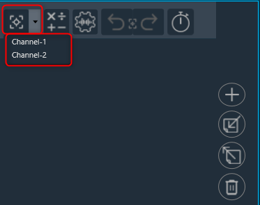
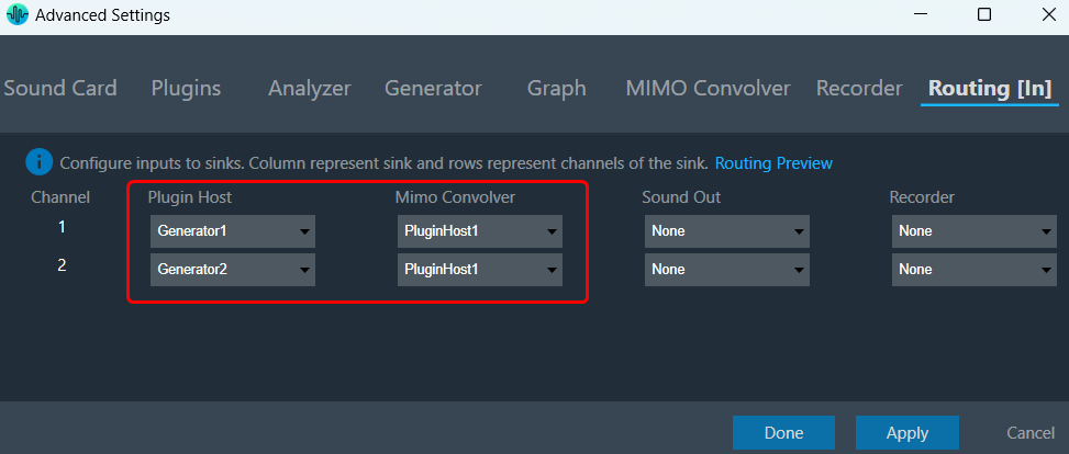
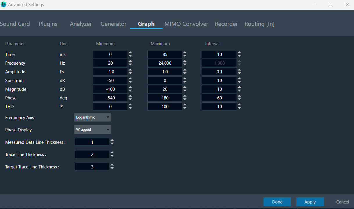
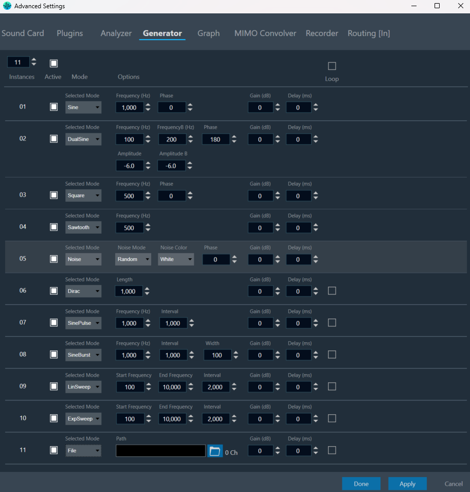
Using the following options, you can configure the graph areas to perform various types of measures.

• Cursor Measurement
• Add Marker
• Add Delta Marker
• Refresh Spectrum
• Capture Graph Image
• Changing Graph Theme
• Zoom To Gates

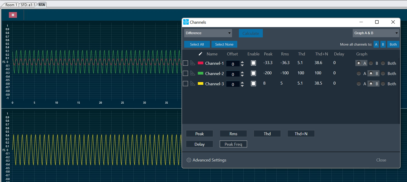
Cursor Measurement

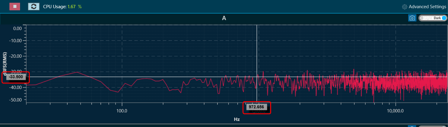
When hovering the mouse over any of the curves or plots on the graph, the horizontal and vertical values of the X and Y positions pointed to will be displayed. It is important to note that while the X value will follow the mouse pointer, the Y value will show the value of the closest trace.

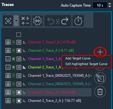
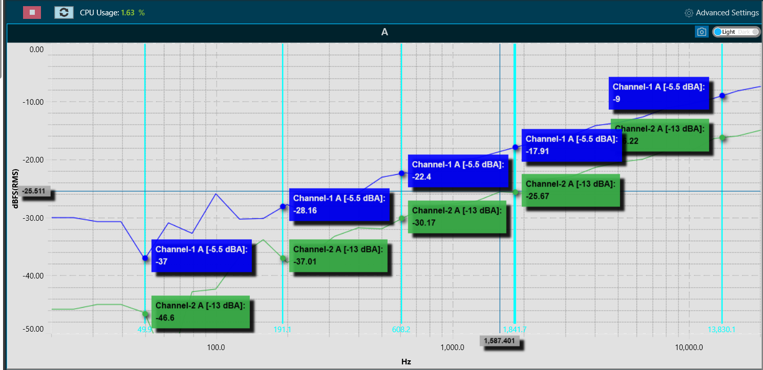
Add Marker

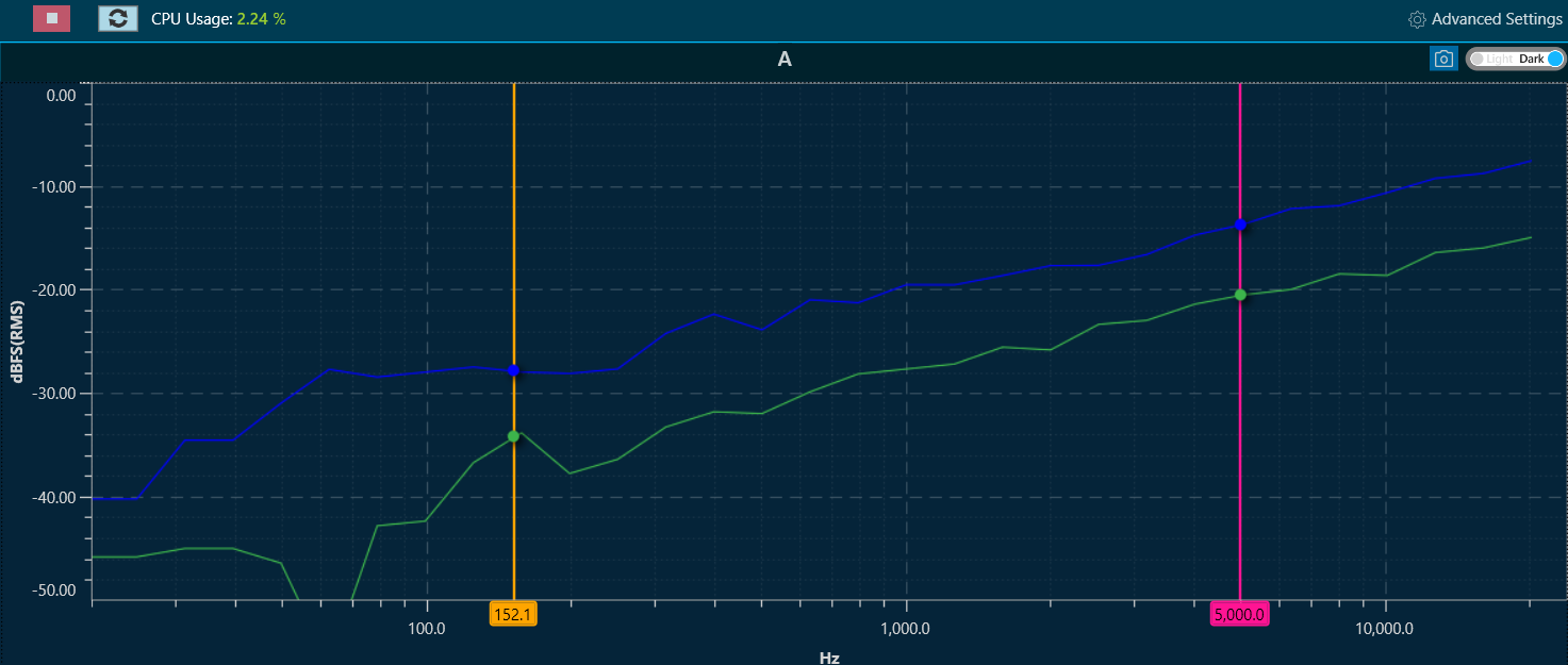
You can mark the curves for value inspection. Press CTRL + click, to create a marker. This marker will display the values of the traces as tooltips on top of the charts. It will show the values of all the traces.

A maximum of 5 markers can be placed on the chart.

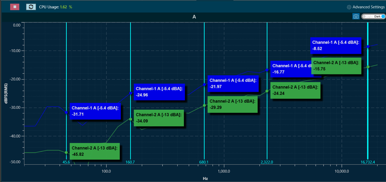
To remove a marker, select the marker by clicking on top of it. The line of the marker will become wider, indicating it has been selected.

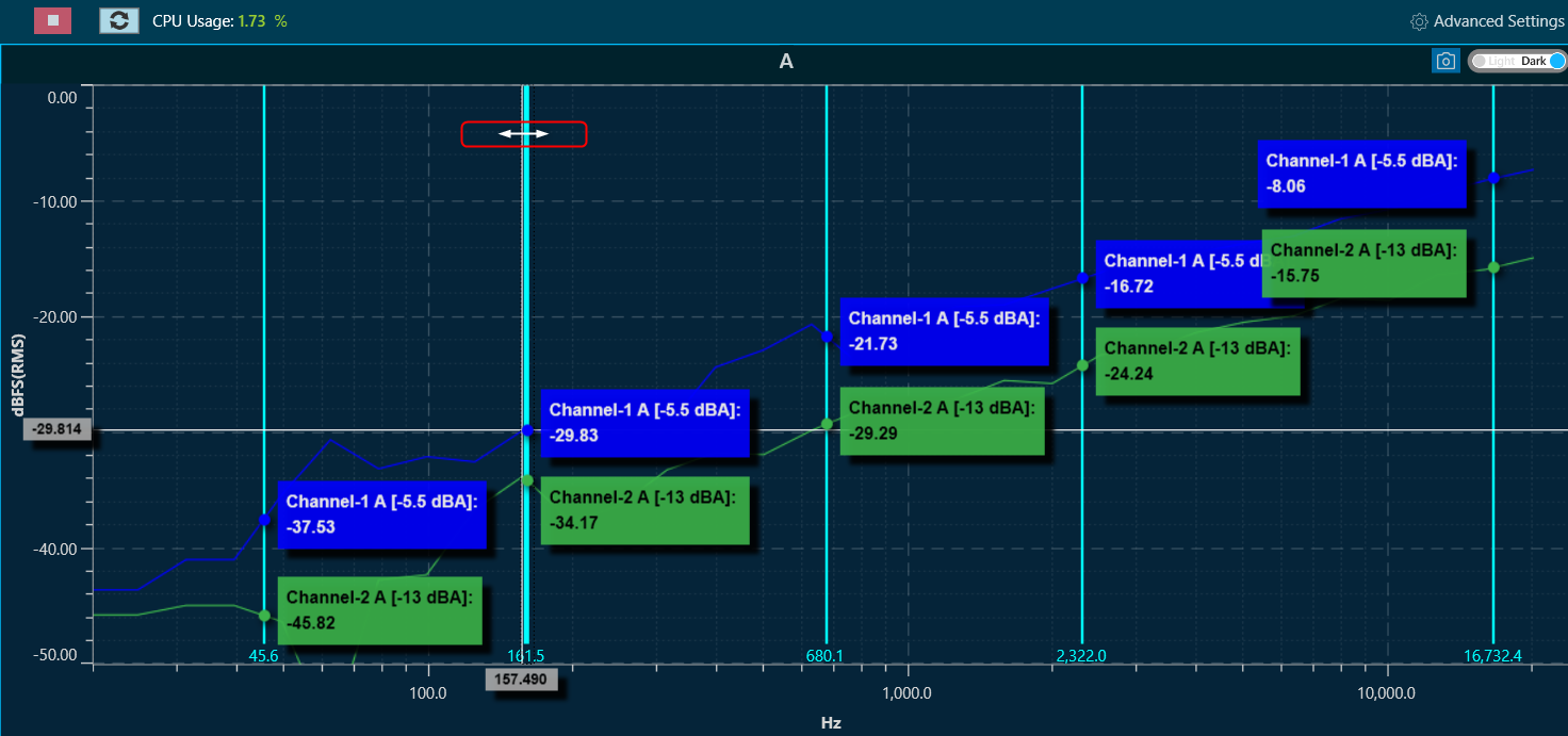
Add Delta Marker

The Delta marker feature helps in createing differential values for selected curves.

To add delta markers, press ALT + click on the chart, and enable measurements from traces where delta values are desired.

The selected traces will display the following information:

• The value at the first marker.
• The value at the second marker.
• The delta (difference) between the markers.

The values are indicated by the trace color and highlighted with the marker color. Delta markers can be dragged to the desired X position.

To disable Delta markers, press ALT + Click again.

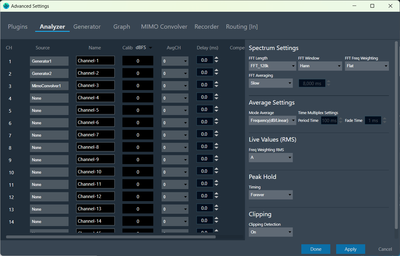
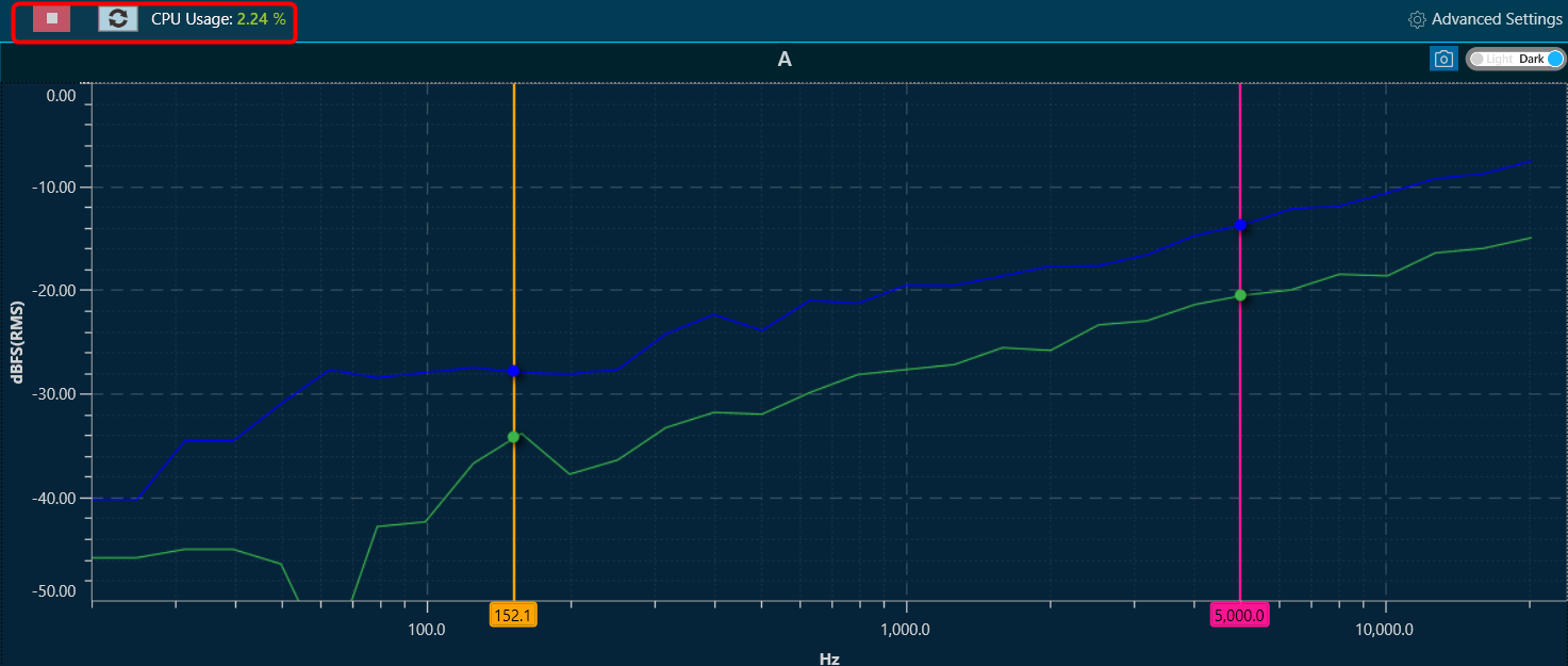
Refresh Spectrum

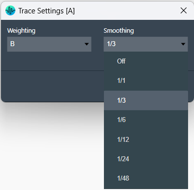
In the spectrum and multiplexer modes, the spectrum refresh button will update all curves displayed, excluding the traces. This functionality allows for the resetting of averaging time periods, which is particularly significant for “forever” averaging.

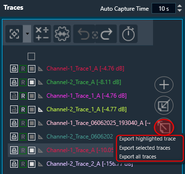
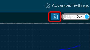
Capture Graph Image

The Export Image feature allows you to export the graphs and certain other details based on the export setting configuration. The exported image file will be available in .png or .jpeg format.
Once you click on the “Export to Image” option, the export setting window for the image will open.

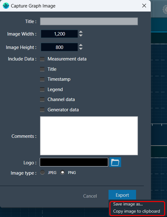
This export setting window includes the following options:

• Title – Enter the image name.
• Image Width – Change the image width.
• Image Height – Change the image height.
• Include Data – Select the option to add various types of data such as Measurement data, Title, Timestamp, Legend, Channel data, and Generator data in the image.
• Comments – Enter the specific comment, that you want to be added to the image.
• Logo – Add the desired logo to the image.
• Image type – Select the image type JPEG or PNG.

Once you configured export settings, click the Export button. The context menu will show you two options, export the image or copy to the clipboard.

• Save image as – option will be opened to save the image to a file.
• Copy the image to the clipboard – will allow you to paste the graph image somewhere else.

Not possible to copy the image to the clipboard for graph B in case of link mode.

The exported image will have the following sections based on the export setting window configuration.

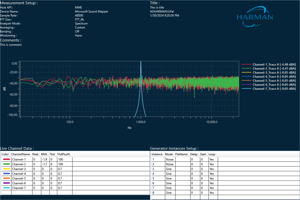
The graph is always present in the exported image. Based on the export setting configuration additional sections like – Measurement information, Title, Time, User details, Logo provided, Live channel data, and Generator instance details are also present in the exported image.

If you select the “Channel data” checkbox, then in the “Legend” live channel entries will not appear, only traces will appear. Otherwise, all items will appear in Legend.

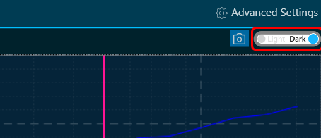
Graph Theme

There is a Toggle button (dark/light theme) in the charts in the RTA graph. Once the Toggle button is clicked, the corresponding custom theme can be selected, and the background of the graph gets changed and vice versa.

Dark Theam

Light Theam

Zoom To Gates

The Zoom To Gates feature allows you to zoom to a specific area in the chart using four gates (two horizontal and two vertical) which you can position by selecting and dragging them to the desired position or if you prefer by placing the value of the position in the chart in the text boxes.

By default, when there are no Curves in chart the values from gates are the limit of visible range of current chart. Only for old projects with that has a loaded curve, the gates will set on the limit of visible range included data.

The Gates are supported for Time, Spectrum, Multiplexer, Phase, Delay and IR modes.

When you move each gate, the current position will be reflected in each value referred to the bottom of the chart identified with a color.

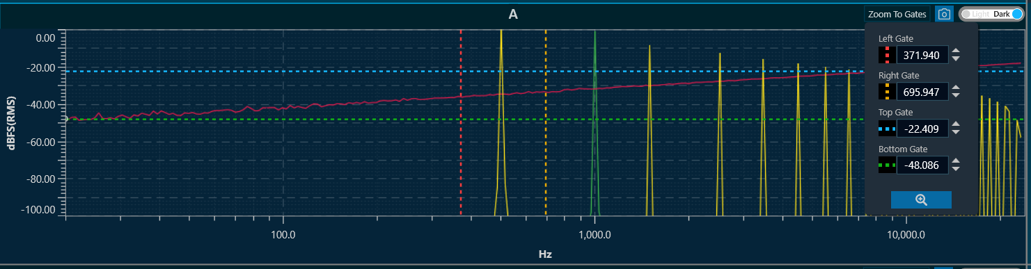
To zoom in on the area between the four lines: Click on the button at the end of the text boxes with the current position values ​​of the gates “Done” and the chart area will automatically position the gates within the limits of the chart and the zoom to the area will have been performed.

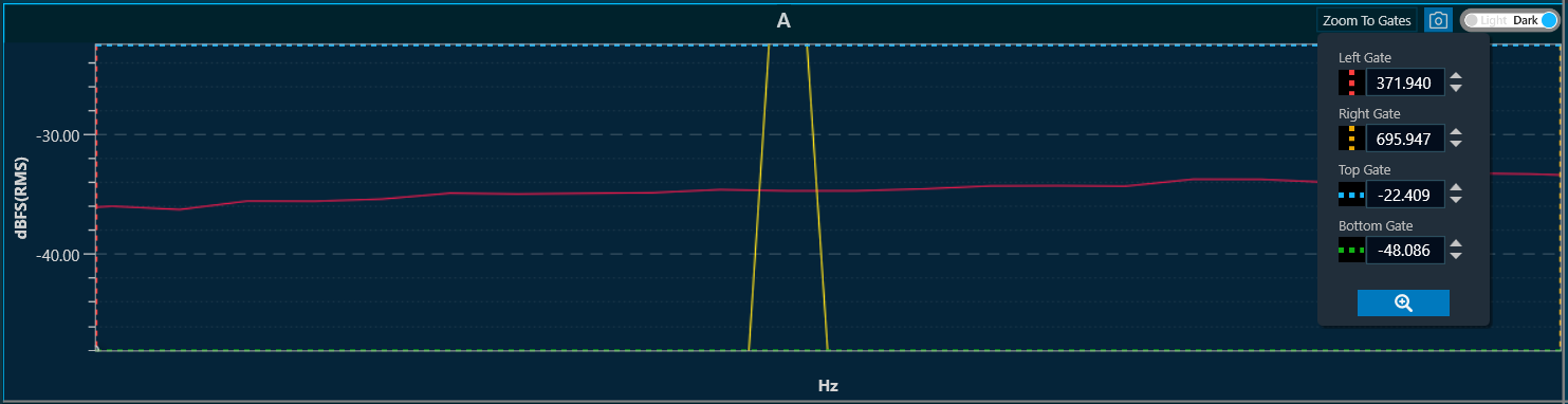
To return to the default value you only have to double click on any area of ​​the chart.

All gate values ​​will be persistent across projects, meaning you can save their last configuration to be exported or used later with specific values.